
Geographical datasets
Pyrocko offers access to commonly used geographical datasets, such as
Topography
The pyrocko.dataset.topo subpackage offers quick access to some
popular global topography datasets.
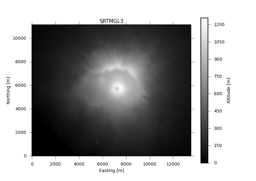
The following example draws gridded topography for Mount Vesuvius from SRTMGL3 ([1], [2], [3], [4]) in local cartesian coordinates.
import numpy as num
from pyrocko import topo, plot, orthodrome as od

lon_min, lon_max, lat_min, lat_max = 14.34, 14.50, 40.77, 40.87
dem_name = 'SRTMGL3'

# extract gridded topography (possibly downloading first)
tile = topo.get(dem_name, (lon_min, lon_max, lat_min, lat_max))

# geographic to local cartesian coordinates
lons = tile.x()
lats = tile.y()
lons2 = num.tile(lons, lats.size)
lats2 = num.repeat(lats, lons.size)
norths, easts = od.latlon_to_ne_numpy(lats[0], lons[0], lats2, lons2)
norths = norths.reshape((lats.size, lons.size))
easts = easts.reshape((lats.size, lons.size))

# plot it
plt = plot.mpl_init(fontsize=10.)
fig = plt.figure(figsize=plot.mpl_papersize('a5', 'landscape'))
axes = fig.add_subplot(1, 1, 1, aspect=1.0)
cbar = axes.pcolormesh(easts, norths, tile.data,
                       cmap='gray', shading='gouraud')
fig.colorbar(cbar).set_label('Altitude [m]')
axes.set_title(dem_name)
axes.set_xlim(easts.min(), easts.max())
axes.set_ylim(norths.min(), norths.max())
axes.set_xlabel('Easting [m]')
axes.set_ylabel('Northing [m]')
fig.savefig('topo_example.png')
Footnotes
| [1] | Farr, T. G., and M. Kobrick, 2000, Shuttle Radar Topography Mission produces a wealth of data. Eos Trans. AGU, 81:583-585. |
| [2] | Farr, T. G. et al., 2007, The Shuttle Radar Topography Mission, Rev. Geophys., 45, RG2004, doi:10.1029/2005RG000183. (Also available online at http://www2.jpl.nasa.gov/srtm/SRTM_paper.pdf) |
| [3] | Kobrick, M., 2006, On the toes of giants-How SRTM was born, Photogramm. Eng. Remote Sens., 72:206-210. |
| [4] | Rosen, P. A. et al., 2000, Synthetic aperture radar interferometry, Proc. IEEE, 88:333-382. |
GSHHG coastal database
The GSHHG database is a high-resolution geography data set. We implement functions to extract coordinates of landmasks.
- Classes covered in this example:
-
import numpy as num
from pyrocko.dataset.gshhg import GSHHG
from matplotlib import pyplot as plt

gshhg = GSHHG.intermediate()
# gshhg = GSHHG.full()
# gshhg = GSHHG.low()

gshhg.is_point_on_land(lat=32.1, lon=44.2)


# Create a landmask for a regular grid
lats = num.linspace(30., 50., 500)
lons = num.linspace(2., 10., 500)

lon_grid, lat_grid = num.meshgrid(lons, lats)
coordinates = num.array([lat_grid.ravel(), lon_grid.ravel()]).T

land_mask = gshhg.get_land_mask(coordinates).reshape(*lat_grid.shape)

plt.pcolormesh(lons, lats, land_mask, cmap='Greys')
plt.show()
Download gshhg_example.py
Footnotes
| [5] | Wessel, P., and W. H. F. Smith, A Global Self-consistent, Hierarchical, High-resolution Shoreline Database, J. Geophys. Res., 101, #B4, pp. 8741-8743, 1996. |
Tectonic plates and boundaries (PB2003)
An updated digital model of plate boundaries [6] offers a global set of present plate boundaries on the Earth. This database used in pyrocko.automap.
- Classes covered in this example:
-
from pyrocko.dataset.tectonics import PeterBird2003

poi_lat = 12.4
poi_lon = 133.5

PB = PeterBird2003()
plates = PB.get_plates()

for plate in plates:
    if plate.contains_point((poi_lat, poi_lon)):
        print(plate.name)
        print(PB.full_name(plate.name))

'''
>>> PS
>>> Philippine Sea Plate
'''
Download tectonics_example.py
Footnotes
| [6] | Bird, Peter. “An updated digital model of plate boundaries.” Geochemistry, Geophysics, Geosystems 4.3 (2003). |
Global strain rate (GSRM1)
Access to the global strain rate data set from Kreemer et al. (2003) [7].
- Classes to be covered in this example:
Warning
To be documented by example!
Footnotes
| [7] | Kreemer, C., W.E. Holt, and A.J. Haines, “An integrated global model of present-day plate motions and plate boundary deformation”, Geophys. J. Int., 154, 8-34, 2003. |