Plotting functions

Generating topographic maps with automap

The pyrocko.plot.automap module provides a painless and clean interface for the Generic Mapping Tool (GMT) [1].

Classes covered in these examples:

• pyrocko.plot.automap.Map

For details on our approach in calling GMT from Python:

• GmtPy - A Python interface to GMT 4/5

Note

To retain PDF transparency in gmtpy use save(psconvert=True).

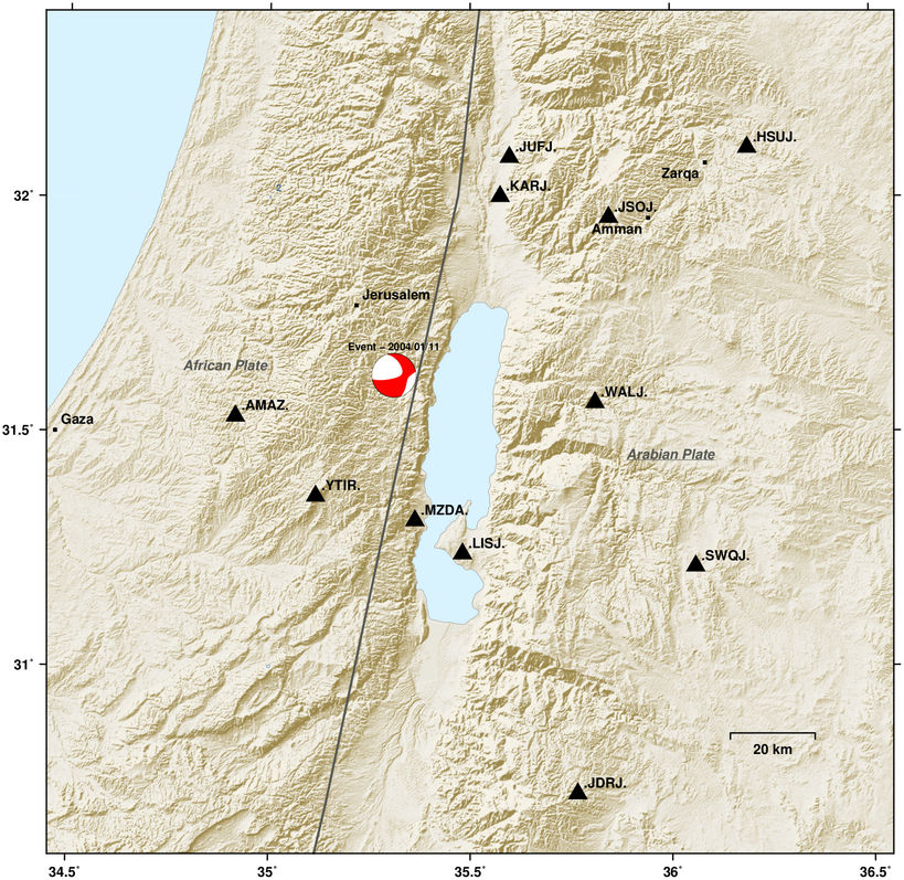
Topographic map of Dead Sea basin

This example demonstrates how to create a map of the Dead Sea area with largest cities, topography and gives a hint on how to access genuine GMT methods.

Download automap_example.py

Station file used in the example: stations_deadsea.pf

from pyrocko.plot.automap import Map
from pyrocko.example import get_example_data
from pyrocko import model, gmtpy
from pyrocko import moment_tensor as pmt

gmtpy.check_have_gmt()

# Download example data
get_example_data('stations_deadsea.pf')
get_example_data('deadsea_events_1976-2017.txt')

# Generate the basic map
m = Map(
    lat=31.5,
    lon=35.5,
    radius=150000.,
    width=30., height=30.,
    show_grid=False,
    show_topo=True,
    color_dry=(238, 236, 230),
    topo_cpt_wet='light_sea_uniform',
    topo_cpt_dry='light_land_uniform',
    illuminate=True,
    illuminate_factor_ocean=0.15,
    show_rivers=False,
    show_plates=True)

# Draw some larger cities covered by the map area
m.draw_cities()

# Generate with latitute, longitude and labels of the stations
stations = model.load_stations('stations_deadsea.pf')
lats = [s.lat for s in stations]
lons = [s.lon for s in stations]
labels = ['.'.join(s.nsl()) for s in stations]

# Stations as black triangles. Genuine GMT commands can be parsed by the maps'
# gmt attribute. Last argument of the psxy function call pipes the maps'
# pojection system.
m.gmt.psxy(in_columns=(lons, lats), S='t20p', G='black', *m.jxyr)

# Station labels
for i in range(len(stations)):
    m.add_label(lats[i], lons[i], labels[i])


# Load events from catalog file (generated using catalog.GlobalCMT()
# download from www.globalcmt.org)
# If no moment tensor is provided in the catalogue, the event is plotted
# as a red circle. Symbol size relative to magnitude.

events = model.load_events('deadsea_events_1976-2017.txt')
beachball_symbol = 'd'
factor_symbl_size = 5.0
for ev in events:
    mag = ev.magnitude
    if ev.moment_tensor is None:
        ev_symb = 'c'+str(mag*factor_symbl_size)+'p'
        m.gmt.psxy(
            in_rows=[[ev.lon, ev.lat]],
            S=ev_symb,
            G=gmtpy.color('scarletred2'),
            W='1p,black',
            *m.jxyr)
    else:
        devi = ev.moment_tensor.deviatoric()
        beachball_size = mag*factor_symbl_size
        mt = devi.m_up_south_east()
        mt = mt / ev.moment_tensor.scalar_moment() \
            * pmt.magnitude_to_moment(5.0)
        m6 = pmt.to6(mt)
        data = (ev.lon, ev.lat, 10) + tuple(m6) + (1, 0, 0)

        if m.gmt.is_gmt5():
            kwargs = dict(
                M=True,
                S='%s%g' % (beachball_symbol[0], (beachball_size) / gmtpy.cm))
        else:
            kwargs = dict(
                S='%s%g' % (beachball_symbol[0],
                            (beachball_size)*2 / gmtpy.cm))

        m.gmt.psmeca(
            in_rows=[data],
            G=gmtpy.color('chocolate1'),
            E='white',
            W='1p,%s' % gmtpy.color('chocolate3'),
            *m.jxyr,
            **kwargs)

m.save('automap_deadsea.png')

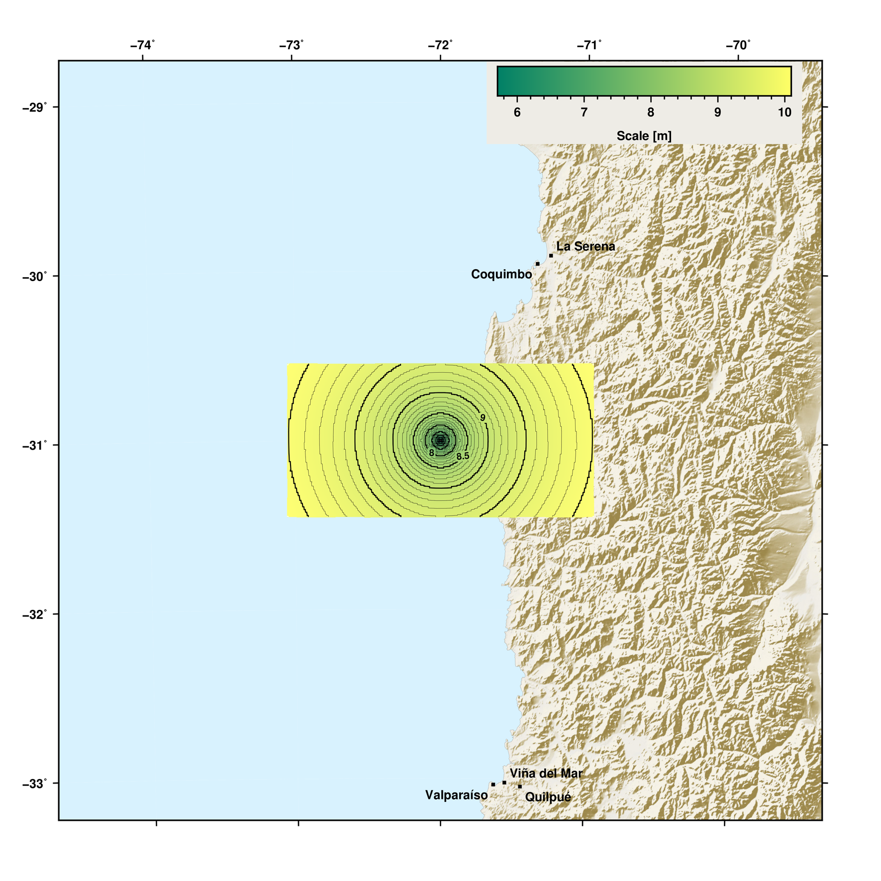
Map with gridded data

This example demonstrates how to create a map using GMT methods and plotting spatial gridded data on it.

Download automap_example2.py

import os

import numpy as num
from scipy.interpolate import RegularGridInterpolator as scrgi

from pyrocko.plot.automap import Map
from pyrocko import gmtpy
import pyrocko.orthodrome as otd

gmtpy.check_have_gmt()
gmt = gmtpy.GMT()

km = 1000.

# Generate the basic map
lat = -31.
lon = -72.
m = Map(
    lat=lat,
    lon=lon,
    radius=250000.,
    width=30., height=30.,
    show_grid=False,
    show_topo=True,
    color_dry=(238, 236, 230),
    topo_cpt_wet='light_sea_uniform',
    topo_cpt_dry='light_land_uniform',
    illuminate=True,
    illuminate_factor_ocean=0.15,
    show_rivers=False,
    show_plates=True)

# Draw some larger cities covered by the map area
m.draw_cities()

# Create grid and data
x = num.linspace(-100., 100., 200) * km
y = num.linspace(-50., 50., 100) * km
yy, xx = num.meshgrid(y, x)

data = num.log10(xx**2 + yy**2)


def extend_1d_coordinate_array(array):
    '''
    Extend 1D coordinate array for gridded data, that grid corners are plotted
    right
    '''
    dx = array[1] - array[0]

    out = num.zeros(array.shape[0] + 2)
    out[1:-1] = array.copy()
    out[0] = array[0] - dx / 2.
    out[-1] = array[-1] + dx / 2.

    return out


def extend_2d_data_array(array):
    '''
    Extend 2D data array for gridded data, that grid corners are plotted
    right
    '''
    out = num.zeros((array.shape[0] + 2, array.shape[1] + 2))
    out[1:-1, 1:-1] = array
    out[1:-1, 0] = array[:, 0]
    out[1:-1, -1] = array[:, -1]
    out[0, 1:-1] = array[0, :]
    out[-1, 1:-1] = array[-1, :]

    for i, j in zip([-1, -1, 0, 0], [-1, 0, -1, 0]):
        out[i, j] = array[i, j]

    return out


def tile_to_length_width(m, ref_lat, ref_lon):
    '''
    Transform grid tile (lat, lon) to easting, northing for data interpolation
    '''
    t, _ = m._get_topo_tile('land')
    grid_lats = t.y()
    grid_lons = t.x()

    meshgrid_lons, meshgrid_lats = num.meshgrid(grid_lons, grid_lats)

    grid_northing, grid_easting = otd.latlon_to_ne_numpy(
        ref_lat, ref_lon, meshgrid_lats.flatten(), meshgrid_lons.flatten())

    return num.hstack((
        grid_easting.reshape(-1, 1), grid_northing.reshape(-1, 1)))


def data_to_grid(m, x, y, data):
    '''
    Create data grid from data and coordinate arrays
    '''
    assert data.shape == (x.shape[0], y.shape[0])

    # Extend grid coordinate and data arrays to plot grid corners right
    x_ext = extend_1d_coordinate_array(x)
    y_ext = extend_1d_coordinate_array(y)
    data_ext = extend_2d_data_array(data)

    # Create grid interpolator based on given coordinates and data
    interpolator = scrgi(
        (x_ext, y_ext),
        data_ext,
        bounds_error=False,
        method='nearest')

    # Interpolate on topography grid from the map
    points_out = tile_to_length_width(m=m, ref_lat=lat, ref_lon=lon)

    t, _ = m._get_topo_tile('land')
    t.data = num.zeros_like(t.data, dtype=num.float)
    t.data[:] = num.nan

    t.data = interpolator(points_out).reshape(t.data.shape)

    # Save grid as grd-file
    gmtpy.savegrd(t.x(), t.y(), t.data, filename='temp.grd', naming='lonlat')


# Create data grid file
data_to_grid(m, x, y, data)

# Create appropiate colormap
increment = (num.max(data) - num.min(data)) / 20.
gmt.makecpt(
    C='0/127.6/102,255/255/102',
    T='%g/%g/%g' % (num.min(data), num.max(data), increment),
    Z=True,
    out_filename='my_cpt.cpt',
    suppress_defaults=True)

# Plot grid image
m.gmt.grdimage(
    'temp.grd',
    C='my_cpt.cpt',
    E='200',
    I='0.1',
    Q=True,
    n='+t0.15',
    *m.jxyr)

# Plot corresponding contour
m.gmt.grdcontour(
    'temp.grd',
    A='0.5',
    C='0.1',
    S='10',
    W='a1.0p',
    *m.jxyr)

# Plot color scake
m.gmt.psscale(
    B='af+lScale [m]',
    C='my_cpt.cpt',
    D='jTR+o1.05c/0.2c+w10c/1c+h',
    F='+g238/236/230',
    *m.jxyr)

# Save plot
m.save('automap_chile.png', resolution=150)

# Clear temporary files
os.remove('temp.grd')
os.remove('my_cpt.cpt')

Footnotes

[1]	Wessel, P., W. H. F. Smith, R. Scharroo, J. F. Luis, and F. Wobbe, Generic Mapping Tools: Improved version released, EOS Trans. AGU, 94, 409-410, 2013.

Plotting beachballs (focal mechanisms)

Classes covered in these examples:

• pyrocko.plot.beachball (visual representation of a focal mechanism)
• pyrocko.moment_tensor (a 3x3 matrix representation of an earthquake source)
• pyrocko.gf.seismosizer.DCSource (a representation of a double couple source object),
• pyrocko.gf.seismosizer.RectangularExplosionSource (a representation of a rectangular explostion source),
• pyrocko.gf.seismosizer.CLVDSource (a representation of a compensated linear vector diploe source object)
• pyrocko.gf.seismosizer.DoubleDCSource (a representation of a double double-couple source object).

Beachballs from moment tensors

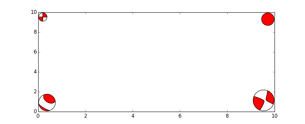
Here we create random moment tensors and plot their beachballs.

Download beachball_example01.py

import random
import logging
from matplotlib import pyplot as plt
from pyrocko import moment_tensor as pmt
from pyrocko import util
from pyrocko.plot import beachball

''' Beachball Copacabana '''

logger = logging.getLogger('pyrocko.examples.beachball_example01')

util.setup_logging()

fig = plt.figure(figsize=(10., 4.))
fig.subplots_adjust(left=0., right=1., bottom=0., top=1.)
axes = fig.add_subplot(1, 1, 1)

for i in range(200):

    # create random moment tensor
    mt = pmt.MomentTensor.random_mt()

    try:
        # create beachball from moment tensor
        beachball.plot_beachball_mpl(
            mt, axes,
            # type of beachball: deviatoric, full or double couple (dc)
            beachball_type='full',
            size=random.random()*120.,
            position=(random.random()*10., random.random()*10.),
            alpha=random.random(),
            linewidth=1.0)

    except beachball.BeachballError as e:
        logger.error('%s for MT:\n%s' % (e, mt))

axes.set_xlim(0., 10.)
axes.set_ylim(0., 10.)
axes.set_axis_off()
fig.savefig('beachball-example01.pdf')

plt.show()

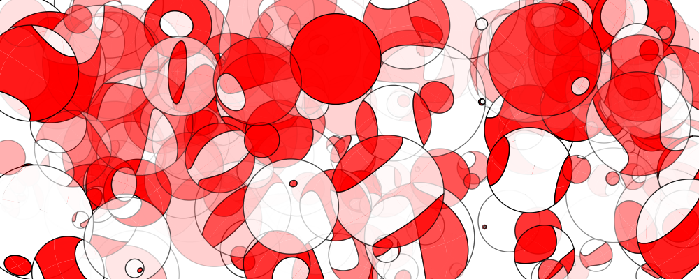
An artistic display of focal mechanisms drawn by classes pyrocko.plot.beachball and pyrocko.moment_tensor.

This example shows how to plot a full, a deviatoric and a double-couple beachball for a moment tensor.

Download beachball_example03.py

from matplotlib import pyplot as plt
from pyrocko import moment_tensor as pmt
from pyrocko import plot


fig = plt.figure(figsize=(4., 2.))
fig.subplots_adjust(left=0., right=1., bottom=0., top=1.)
axes = fig.add_subplot(1, 1, 1)
axes.set_xlim(0., 4.)
axes.set_ylim(0., 2.)
axes.set_axis_off()

for i, beachball_type in enumerate(['full', 'deviatoric', 'dc']):
    plot.beachball.plot_beachball_mpl(
            pmt.as_mt((124654616., 370943136., -6965434.0,
                       553316224., -307467264., 84703760.0)),
            axes,
            beachball_type=beachball_type,
            size=60.,
            position=(i+1, 1),
            color_t=plot.mpl_color('scarletred2'),
            linewidth=1.0)

fig.savefig('beachball-example03.pdf')
plt.show()

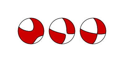
The three types of beachballs that can be plotted through pyrocko.

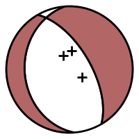
Beachballs from source objects

This example shows how to add beachballs of various sizes to the corners of a plot by obtaining the moment tensor from four different source object types: pyrocko.gf.seismosizer.DCSource (upper left), pyrocko.gf.seismosizer.RectangularExplosionSource (upper right), pyrocko.gf.seismosizer.CLVDSource (lower left) and pyrocko.gf.seismosizer.DoubleDCSource (lower right).

Creating the beachball this ways allows for finer control over their location based on their size (in display units) which allows for a round beachball even if the axis are not 1:1.

Download beachball_example02.py

from matplotlib import transforms, pyplot as plt
from pyrocko import gf
from pyrocko.plot import beachball


# create source object
source1 = gf.DCSource(depth=35e3, strike=0., dip=90., rake=0.)

# set size of beachball
sz = 20.
# set beachball offset in points (one point from each axis)
szpt = (sz / 2.) / 72. + 1. / 72.

fig = plt.figure(figsize=(10., 4.))
ax = fig.add_subplot(1, 1, 1)
ax.set_xlim(0, 10)
ax.set_ylim(0, 10)

# get the bounding point (left-top)
x0 = ax.get_xlim()[0]
y1 = ax.get_ylim()[1]

# create a translation matrix, based on the final figure size and
# beachball location
move_trans = transforms.ScaledTranslation(szpt, -szpt, fig.dpi_scale_trans)

# get the inverse matrix for the axis where the beachball will be plotted
inv_trans = ax.transData.inverted()

# set the bouding point relative to the plotted axis of the beachball
x0, y1 = inv_trans.transform(move_trans.transform(
    ax.transData.transform((x0, y1))))

# plot beachball
beachball.plot_beachball_mpl(source1.pyrocko_moment_tensor(), ax,
                             beachball_type='full', size=sz,
                             position=(x0, y1), linewidth=1.)


# create source object
source2 = gf.RectangularExplosionSource(depth=35e3, strike=0., dip=90.)

# set size of beachball
sz = 30.
# set beachball offset in points (one point from each axis)
szpt = (sz / 2.) / 72. + 1. / 72.

# get the bounding point (right-upper)
x1 = ax.get_xlim()[1]
y1 = ax.get_ylim()[1]

# create a translation matrix, based on the final figure size and
# beachball location
move_trans = transforms.ScaledTranslation(-szpt, -szpt, fig.dpi_scale_trans)

# get the inverse matrix for the axis where the beachball will be plotted
inv_trans = ax.transData.inverted()

# set the bouding point relative to the plotted axis of the beachball
x1, y1 = inv_trans.transform(move_trans.transform(
    ax.transData.transform((x1, y1))))

# plot beachball
beachball.plot_beachball_mpl(source2.pyrocko_moment_tensor(), ax,
                             beachball_type='full', size=sz,
                             position=(x1, y1), linewidth=1.)


# create source object
source3 = gf.CLVDSource(moment=1.0, azimuth=30., dip=30.)

# set size of beachball
sz = 40.
# set beachball offset in points (one point from each axis)
szpt = (sz / 2.) / 72. + 1. / 72.

# get the bounding point (left-bottom)
x0 = ax.get_xlim()[0]
y0 = ax.get_ylim()[0]

# create a translation matrix, based on the final figure size and
# beachball location
move_trans = transforms.ScaledTranslation(szpt, szpt, fig.dpi_scale_trans)

# get the inverse matrix for the axis where the beachball will be plotted
inv_trans = ax.transData.inverted()

# set the bouding point relative to the plotted axis of the beachball
x0, y0 = inv_trans.transform(move_trans.transform(
    ax.transData.transform((x0, y0))))

# plot beachball
beachball.plot_beachball_mpl(source3.pyrocko_moment_tensor(), ax,
                             beachball_type='full', size=sz,
                             position=(x0, y0), linewidth=1.)

# create source object
source4 = gf.DoubleDCSource(depth=35e3, strike1=0., dip1=90., rake1=0.,
                            strike2=45., dip2=74., rake2=0.)

# set size of beachball
sz = 50.
# set beachball offset in points (one point from each axis)
szpt = (sz / 2.) / 72. + 1. / 72.

# get the bounding point (right-bottom)
x1 = ax.get_xlim()[1]
y0 = ax.get_ylim()[0]

# create a translation matrix, based on the final figure size and
# beachball location
move_trans = transforms.ScaledTranslation(-szpt, szpt, fig.dpi_scale_trans)

# get the inverse matrix for the axis where the beachball will be plotted
inv_trans = ax.transData.inverted()

# set the bouding point relative to the plotted axis of the beachball
x1, y0 = inv_trans.transform(move_trans.transform(
    ax.transData.transform((x1, y0))))

# plot beachball
beachball.plot_beachball_mpl(source4.pyrocko_moment_tensor(), ax,
                             beachball_type='full', size=sz,
                             position=(x1, y0), linewidth=1.)

fig.savefig('beachball-example02.pdf')
plt.show()

Four different source object types plotted with different beachball sizes.

Fuzzy beachballs with uncertainty

If we want to express moment tensor uncertainties we can plot fuzzy beachballs from an ensemble of many solutions.

This example will generate random solution around a best moment tensor (red lines). The perturbed solutions are the uncertainty which can be illustrated in a fuzzy beachball.

Download beachball_example05.py

from pyrocko.plot import beachball
import pyrocko.moment_tensor as mtm

import numpy as num
from matplotlib import pyplot as plt


fig = plt.figure(figsize=(4., 4.))
fig.subplots_adjust(left=0., right=1., bottom=0., top=1.)
axes = fig.add_subplot(1, 1, 1)

# Number of available solutions
n_balls = 1000

# Best solution
strike = 135.
dip = 65.
rake = 15.

best_mt = mtm.MomentTensor.from_values((strike, dip, rake))


def get_random_uniform(lower, upper, dimension=1):
    ''' Help function to pertubate the best solution '''
    return (upper - lower) * num.random.rand(dimension) + lower


mts = []
for i in range(n_balls):
    strike_dev = get_random_uniform(-15., 15.)
    mts.append(mtm.MomentTensor.from_values(
        (strike + strike_dev, dip, rake)))

plot_kwargs = {
    'beachball_type': 'full',
    'size': 8,
    'position': (5, 5),
    'color_t': 'black',
    'edgecolor': 'black'
    }

beachball.plot_fuzzy_beachball_mpl_pixmap(mts, axes, best_mt, **plot_kwargs)

# Decorate the axes
axes.set_xlim(0., 10.)
axes.set_ylim(0., 10.)
axes.set_axis_off()

plt.show()

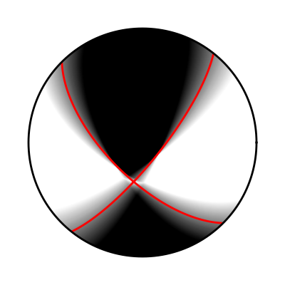
Fuzzy beachball illustrating the solutions uncertainty.

Beachballs views for cross-sections:

It is useful to show beachballs from other view angles, as in cross-sections. For that, we can define a view for all beachball plotting functions as shown here:

Download beachball_example06.py

#!/usr/bin/env python3

from matplotlib import pyplot as plt
from pyrocko import moment_tensor as pmt
from pyrocko.plot import beachball

mt = pmt.as_mt([0.424, -0.47, 0.33, 0.711, -0.09, 0.16])
axes = plt.gca()

beachball.plot_beachball_mpl(
    mt, axes,
    size=50.,
    position=(0., 0.),
    view='top')

beachball.plot_beachball_mpl(
    mt, axes,
    size=50.,
    position=(0, -1.),
    view='south')

beachball.plot_beachball_mpl(
    mt, axes,
    size=50.,
    position=(-1, 0.),
    view='east')

beachball.plot_beachball_mpl(
    mt, axes,
    size=50.,
    position=(0, 1.),
    view='north')

beachball.plot_beachball_mpl(
    mt, axes,
    size=50.,
    position=(1, 0.),
    view='west')

axes.set_xlim(-2., 2.)
axes.set_ylim(-2., 2.)
plt.show()

Add station symbols to focal sphere diagram

This example shows how to add station symbols at the positions where P wave rays pierce the focal sphere.

The function to plot focal spheres (pyrocko.plot.beachball.plot_beachball_mpl()) uses the function pyrocko.plot.beachball.project() in the final projection from 3D to 2D coordinates. Here we use this function to place additional symbols on the plot. The take-off angles needed can be computed with some help of the pyrocko.cake module. Azimuth and distance computations are done with functions from pyrocko.orthodrome.

Download beachball_example04.py

import numpy as num
from matplotlib import pyplot as plt
from pyrocko import moment_tensor as pmt, cake, orthodrome
from pyrocko.plot import beachball

km = 1000.

# source position and mechanism
slat, slon, sdepth = 0., 0., 10.*km
mt = pmt.MomentTensor.random_dc()

# receiver positions
rdepth = 0.0
rlatlons = [(50., 10.), (60., -50.), (-30., 60.)]

# earth model and phase for takeoff angle computations
mod = cake.load_model('ak135-f-continental.m')
phases = cake.PhaseDef.classic('P')

# setup figure with aspect=1.0/1.0, ranges=[-1.1, 1.1]
fig = plt.figure(figsize=(2., 2.))  # size in inch
fig.subplots_adjust(left=0., right=1., bottom=0., top=1.)
axes = fig.add_subplot(1, 1, 1, aspect=1.0)
axes.set_axis_off()
axes.set_xlim(-1.1, 1.1)
axes.set_ylim(-1.1, 1.1)

projection = 'lambert'

beachball.plot_beachball_mpl(
    mt, axes,
    position=(0., 0.),
    size=2.0,
    color_t=(0.7, 0.4, 0.4),
    projection=projection,
    size_units='data')

for rlat, rlon in rlatlons:
    distance = orthodrome.distance_accurate50m(slat, slon, rlat, rlon)
    rays = mod.arrivals(
        phases=cake.PhaseDef('P'),
        zstart=sdepth, zstop=rdepth, distances=[distance*cake.m2d])

    if not rays:
        continue

    takeoff = rays[0].takeoff_angle()
    azi = orthodrome.azimuth(slat, slon, rlat, rlon)

    # to spherical coordinates, r, theta, phi in radians
    rtp = num.array([[1., num.deg2rad(takeoff), num.deg2rad(90.-azi)]])

    # to 3D coordinates (x, y, z)
    points = beachball.numpy_rtp2xyz(rtp)

    # project to 2D with same projection as used in beachball
    x, y = beachball.project(points, projection=projection).T

    axes.plot(x, y, '+', ms=10., mew=2.0, mec='black', mfc='none')

fig.savefig('beachball-example04.png')

Focal sphere diagram with markers at positions of P wave ray piercing points.

Hudson’s source type plot

Hudson’s source type plot [Hudson, 1989] is a way to visually represent the widely used “standard” decomposition of a moment tensor into its isotropic, its compensated linear vector dipole (CLVD), and its double-couple (DC) components.

The function pyrocko.plot.hudson.project() may be used to get the (u,v) coordinates for a given (full) moment tensor used for positioning the symbol in the plot. The function pyrocko.plot.hudson.draw_axes() can be used to conveniently draw the axes and annotions. Note, that we follow the original convention introduced by Hudson, to place the negative CLVD on the right hand side.

Download hudson_diagram.py

from __future__ import print_function
import sys
from matplotlib import pyplot as plt
from pyrocko.plot import hudson, beachball, mpl_init, mpl_color
from pyrocko import moment_tensor as pmt

# a bunch of random MTs
moment_tensors = [pmt.random_mt() for _ in range(200)]

# setup plot layout
fontsize = 10.
markersize = fontsize
mpl_init(fontsize=fontsize)
width = 7.
figsize = (width, width / (4. / 3.))
fig = plt.figure(figsize=figsize)
axes = fig.add_subplot(1, 1, 1)
fig.subplots_adjust(left=0.03, right=0.97, bottom=0.03, top=0.97)

# draw focal sphere diagrams for the random MTs
for mt in moment_tensors:
    u, v = hudson.project(mt)
    try:
        beachball.plot_beachball_mpl(
            mt, axes,
            beachball_type='full',
            position=(u, v),
            size=markersize,
            color_t=mpl_color('skyblue3'),
            color_p=mpl_color('skyblue1'),
            alpha=1.0,  # < 1 for transparency
            zorder=1,
            linewidth=0.25)

    except beachball.BeachballError as e:
        print(str(e), file=sys.stderr)

# draw the axes and annotations of the hudson plot
hudson.draw_axes(axes)

fig.savefig('hudson_diagram.png', dpi=150)
# plt.show()

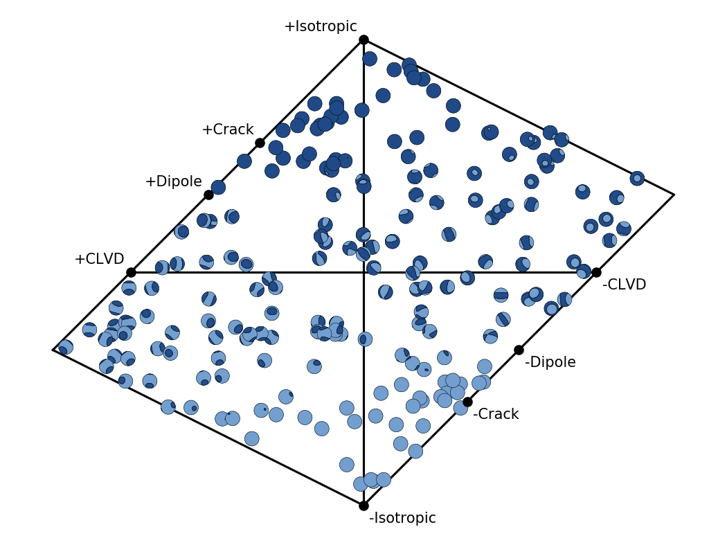
Hudson’s source type plot for 200 random moment tensors.