plot.beachball

exception BeachballError

class FixedPointOffsetTransform(trans, dpi_scale_trans, fixed_point)

transform_non_affine(values)

Performs only the non-affine part of the transformation.

transform(values) is always equivalent to transform_affine(transform_non_affine(values)).

In non-affine transformations, this is generally equivalent to transform(values). In affine transformations, this is always a no-op.

Accepts a numpy array of shape (N x input_dims) and returns a numpy array of shape (N x output_dims).

Alternatively, accepts a numpy array of length input_dims and returns a numpy array of length output_dims.

plot_beachball_mpl(mt, axes, beachball_type='deviatoric', position=(0.0, 0.0), size=None, zorder=0, color_t='red', color_p='white', edgecolor='black', linewidth=2, alpha=1.0, arcres=181, decimation=1, projection='lambert', size_units='points', view='top')

Plot beachball diagram to a Matplotlib plot

Parameters:

• mt – pyrocko.moment_tensor.MomentTensor object or an array or sequence which can be converted into an MT object
• beachball_type – 'deviatoric' (default), 'full', or 'dc'
• position – position of the beachball in data coordinates
• size – diameter of the beachball either in points or in data coordinates, depending on the size_units setting
• zorder – (passed through to matplotlib drawing functions)
• color_t – color for compressional quadrants (default: 'red')
• color_p – color for extensive quadrants (default: 'white')
• edgecolor – color for lines (default: 'black')
• linewidth – linewidth in points (default: 2)
• alpha – (passed through to matplotlib drawing functions)
• projection – 'lambert' (default), 'stereographic', or 'orthographic'
• size_units – 'points' (default) or 'data', where the latter causes the beachball to be projected in the plots data coordinates (axes must have an aspect ratio of 1.0 or the beachball will be shown distorted when using this).
• view – View the beachball from top, north, south, east or west. Useful for to show beachballs in cross-sections. Default is top.

plot_fuzzy_beachball_mpl_pixmap(mts, axes, best_mt=None, beachball_type='deviatoric', position=(0.0, 0.0), size=None, zorder=0, color_t='red', color_p='white', edgecolor='black', best_color='red', linewidth=2, alpha=1.0, projection='lambert', size_units='data', grid_resolution=200, method='imshow', view='top')

Plot fuzzy beachball from a list of given MomentTensors

Parameters:

• mts – list of pyrocko.moment_tensor.MomentTensor object or an array or sequence which can be converted into an MT object
• best_mt – pyrocko.moment_tensor.MomentTensor object or an array or sequence which can be converted into an MT object of most likely or minimum misfit solution to extra highlight
• best_color – mpl color for best MomentTensor edges, polygons are not plotted

See plot_beachball_mpl for other arguments

plot.cake_plot

path2colorint(path)

Calculate an integer representation deduced from path’s given name.

plot.hudson

project(mt)

Calculate Hudson’s (u, v) coordinates for a given moment tensor.

The moment tensor can be given as a pyrocko.moment_tensor.MomentTensor object, or by anything that can be converted to a 3x3 NumPy matrix, or as the six independent moment tensor entries as (mnn, mee, mdd, mne, mnd, med).

draw_axes(axes, color='black', fontsize=12, linewidth=1.5)

Plot axes and annotations of Hudson’s MT decomposition diagram.

plot.response

This module contains functions to plot instrument response transfer functions in Bode plot style using Matplotlib.

Example

• test_response_plot.py

from pyrocko.plot import response
from pyrocko.example import get_example_data

get_example_data('test_response.resp')

resps, labels = response.load_response_information(
    'test_response.resp', 'resp')

response.plot(
    responses=resps, labels=labels, filename='test_response.png',
    fmin=0.001, fmax=400., dpi=75.)

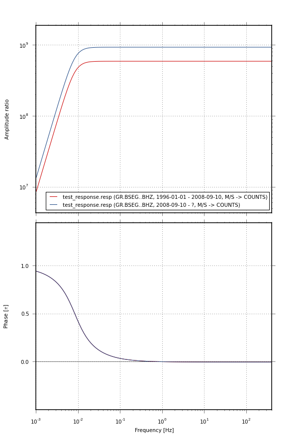
Example response plot

draw(response, axes_amplitude=None, axes_phase=None, fmin=0.01, fmax=100.0, nf=100, normalize=False, style={}, label=None)

Draw instrument response in Bode plot style to given Matplotlib axes

Parameters:

• response – instrument response as a pyrocko.trace.FrequencyResponse object
• axes_amplitude – matplotlib.axes.Axes object to use when drawing the amplitude response
• axes_phase – matplotlib.axes.Axes object to use when drawing the phase response
• fmin – minimum frequency [Hz]
• fmax – maximum frequency [Hz]
• nf – number of frequencies where to evaluate the response
• style – dict with keyword arguments to tune the line style
• label – string to be passed to the label argument of matplotlib.axes.Axes.plot()

setup_axes(axes_amplitude=None, axes_phase=None)

Configure axes in Bode plot style.

plot(responses, filename=None, dpi=100, fmin=0.01, fmax=100.0, nf=100, normalize=False, fontsize=10.0, figsize=None, styles=None, labels=None)

Draw instrument responses in Bode plot style.

Parameters:

• responses – instrument responses as pyrocko.trace.FrequencyResponse objects
• fmin – minimum frequency [Hz]
• fmax – maximum frequency [Hz]
• nf – number of frequencies where to evaluate the response
• normalize – if True normalize flat part of response to be 1
• styles – list of dict objects with keyword arguments to be passed to matplotlib’s matplotlib.axes.Axes.plot() function when drawing the response lines. Length must match number of responses.
• filename – file name to pass to matplotlib’s savefig function. If None, the plot is shown with matplotlib.pyplot.show().
• fontsize – font size in points used in axis labels and legend
• figsize – tuple, (width, height) in inches
• labels – list of names to show in legend. Length must correspond to number of responses.

plot.directivity

plot_directivity(engine, source, store_id, distance=300000.0, azi_begin=0.0, azi_end=360.0, dazi=1.0, phase_begin='first{stored:any_P}-10%', phase_end='last{stored:any_S}+50', quantity='displacement', envelope=False, component='R', fmin=0.01, fmax=0.1, hillshade=True, cmap=None, plot_mt='full', show_phases=True, show_description=True, reverse_time=False, show_nucleations=True, axes=None, nthreads=0)

Plot the directivity and radiation characteristics of source models

Synthetic seismic traces (R, T or Z) are forward-modelled at a defined radius, covering the full or partial azimuthal range and projected on a polar plot. Difference in the amplitude are enhanced by hillshading the data.

Parameters:

• engine (Engine) – Forward modelling engine
• source (Source) – Parametrized source model
• store_id (str) – Store ID used for forward modelling
• distance (float) – Distance in [m]
• azi_begin (float) – Begin azimuth in [deg]
• azi_end (float) – End azimuth in [deg]
• dazi (float) – Delta azimuth, bin size [deg]
• phase_begin (Timing) – Start time of the window
• phase_end (Timing) – End time of the window
• quantity (str) – Seismogram quantity, default displacement
• envelope (bool) – Plot envelop instead of seismic trace
• component (str) – Forward modelled component, default R. Choose from RTZ
• fmin (float) – Bandpass lower frequency [Hz], default 0.01
• fmax (float) – Bandpass upper frequency [Hz], default 0.1
• hillshade (bool) – Enable hillshading, default True
• cmap (str) – Matplotlit colormap to use, default seismic. When envelope is True the default colormap will be Reds.
• plot_mt (str, bool) – Plot a centered moment tensor, default full. Choose from full, deviatoric, dc or False
• show_phases (bool) – Show annotations, default True
• show_description (bool) – Show desciption, default True
• reverse_time (bool) – Reverse time axis. First phases arrive at the center, default False
• show_nucleations (bool) – Show nucleation piercing points on the moment tensor, default True
• axes (matplotlib.axes.Axes) – Give axes to plot into
• nthreads (int) – Number of threads used for forward modelling, default 0 - all available cores