beachball

exception BeachballError

plot_beachball_mpl(mt, axes, beachball_type='deviatoric', position=(0.0, 0.0), size=None, zorder=0, color_t='red', color_p='white', edgecolor='black', linewidth=2, alpha=1.0, arcres=181, decimation=1, projection='lambert', size_units='points', view='top')

Plot beachball diagram to a Matplotlib plot

Parameters:

• mt – pyrocko.moment_tensor.MomentTensor object or an array or sequence which can be converted into an MT object

• beachball_type – 'deviatoric' (default), 'full', or 'dc'

• position – position of the beachball in data coordinates

• size – diameter of the beachball either in points or in data coordinates, depending on the size_units setting

• zorder – (passed through to matplotlib drawing functions)

• color_t – color for compressional quadrants (default: 'red')

• color_p – color for extensive quadrants (default: 'white')

• edgecolor – color for lines (default: 'black')

• linewidth – linewidth in points (default: 2)

• alpha – (passed through to matplotlib drawing functions)

• projection – 'lambert' (default), 'stereographic', or 'orthographic'

• size_units – 'points' (default) or 'data', where the latter causes the beachball to be projected in the plots data coordinates (axes must have an aspect ratio of 1.0 or the beachball will be shown distorted when using this).

• view – View the beachball from 'top', 'north', 'south', 'east' or 'west', or project onto plane given by (strike, dip). Useful to show beachballs in cross-sections. Default is 'top'.

plot_fuzzy_beachball_mpl_pixmap(mts, axes, best_mt=None, beachball_type='deviatoric', position=(0.0, 0.0), size=None, zorder=0, color_t='red', color_p='white', edgecolor='black', best_color='red', linewidth=2, alpha=1.0, projection='lambert', size_units='data', grid_resolution=200, method='imshow', view='top')

Plot fuzzy beachball from a list of given MomentTensors

Parameters:

• mts – list of pyrocko.moment_tensor.MomentTensor object or an array or sequence which can be converted into an MT object

• best_mt – pyrocko.moment_tensor.MomentTensor object or an array or sequence which can be converted into an MT object of most likely or minimum misfit solution to extra highlight

• best_color – mpl color for best MomentTensor edges, polygons are not plotted

See plot_beachball_mpl for other arguments

cake_plot

path2colorint(path)

Calculate an integer representation deduced from path’s given name.

hudson

project(mt)

Calculate Hudson’s (u, v) coordinates for a given moment tensor.

The moment tensor can be given as a pyrocko.moment_tensor.MomentTensor object, or by anything that can be converted to a 3x3 NumPy matrix, or as the six independent moment tensor entries as (mnn, mee, mdd, mne, mnd, med).

draw_axes(axes, color='black', fontsize=12, linewidth=1.5)

Plot axes and annotations of Hudson’s MT decomposition diagram.

response

This module contains functions to plot instrument response transfer functions in Bode plot style using Matplotlib.

Example

• test_response_plot.py

from pyrocko.plot import response
from pyrocko.example import get_example_data

get_example_data('test_response.resp')

resps, labels = response.load_response_information(
    'test_response.resp', 'resp')

response.plot(
    responses=resps, labels=labels, filename='test_response.png',
    fmin=0.001, fmax=400., dpi=75.)

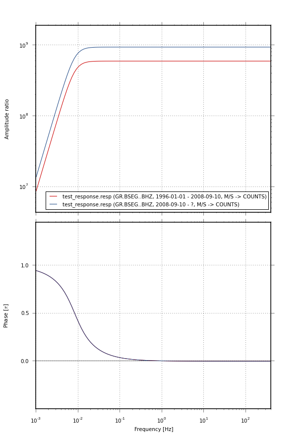
Example response plot

draw(response, axes_amplitude=None, axes_phase=None, fmin=0.01, fmax=100.0, nf=100, normalize=False, style={}, label=None, show_breakpoints=False, color_pool=None, label_pool=None)

Draw instrument response in Bode plot style to given Matplotlib axes

Parameters:

• response – instrument response as a pyrocko.response.FrequencyResponse object

• axes_amplitude – matplotlib.axes.Axes object to use when drawing the amplitude response

• axes_phase – matplotlib.axes.Axes object to use when drawing the phase response

• fmin – minimum frequency [Hz]

• fmax – maximum frequency [Hz]

• nf – number of frequencies where to evaluate the response

• style – dict with keyword arguments to tune the line style

• label – string to be passed to the label argument of matplotlib.axes.Axes.plot()

setup_axes(axes_amplitude=None, axes_phase=None)

Configure axes in Bode plot style.

plot(responses, filename=None, dpi=100, fmin=0.01, fmax=100.0, nf=100, normalize=False, fontsize=10.0, figsize=None, styles=None, labels=None, show_breakpoints=False, separate_combined_labels=None)

Draw instrument responses in Bode plot style.

Parameters:

• responses – instrument responses as pyrocko.response.FrequencyResponse objects

• fmin – minimum frequency [Hz]

• fmax – maximum frequency [Hz]

• nf – number of frequencies where to evaluate the response

• normalize – if True normalize flat part of response to be 1

• styles – list of dict objects with keyword arguments to be passed to matplotlib’s matplotlib.axes.Axes.plot() function when drawing the response lines. Length must match number of responses.

• filename – file name to pass to matplotlib’s savefig function. If None, the plot is shown with matplotlib.pyplot.show().

• fontsize – font size in points used in axis labels and legend

• figsize – tuple, (width, height) in inches

• labels – list of names to show in legend. Length must correspond to number of responses.

• show_breakpoints – show breakpoints of pole-zero responses.

directivity

plot_directivity(engine, source, store_id, distance=300000.0, azi_begin=0.0, azi_end=360.0, dazi=1.0, phases={'P': 'first{stored:any_P}-10%', 'S': 'last{stored:any_S}+50'}, interpolation='multilinear', target_depth=0.0, quantity='displacement', envelope=False, component='R', fmin=0.01, fmax=0.1, hillshade=True, cmap=None, plot_mt='full', show_phases=True, show_description=True, reverse_time=False, show_nucleations=True, axes=None, nthreads=0)

Plot the directivity and radiation characteristics of source models.

Synthetic seismic traces (R, T or Z) are forward-modelled at a defined radius, covering the full or partial azimuthal range and projected on a polar plot. Difference in the amplitude are enhanced by hillshading the data.

Parameters:

• engine (Engine) – Forward modelling engine

• source (Source) – Parametrized source model

• store_id (str) – Store ID used for forward modelling

• distance (float) – Distance in [m]

• azi_begin (float) – Begin azimuth in [deg]

• azi_end (float) – End azimuth in [deg]

• dazi (float) – Delta azimuth, bin size [deg]

• phases (dict with str keys and Timing values) – Phases to define start and end of time window

• quantity (str) – Seismogram quantity, default displacement

• envelope (bool) – Plot envelope instead of seismic trace

• component (str) – Forward modelled component, default R. Choose from RTZ

• fmin (float) – Bandpass lower frequency [Hz], default 0.01

• fmax (float) – Bandpass upper frequency [Hz], default 0.1

• hillshade (bool) – Enable hillshading, default True

• cmap (str) – Matplotlib colormap to use, default seismic. When envelope is True the default colormap will be Reds.

• plot_mt (str, bool) – Plot a centered moment tensor, default full. Choose from full, deviatoric, dc or False

• show_phases (bool) – Show annotations, default True

• show_description (bool) – Show description, default True

• reverse_time (bool) – Reverse time axis. First phases arrive at the center, default False

• show_nucleations (bool) – Show nucleation piercing points on the moment tensor, default True

• axes (matplotlib.axes.Axes) – Give axes to plot into

• nthreads (int) – Number of threads used for forward modelling, default 0 - all available cores

dynamic_rupture

make_colormap(gmt, vmin, vmax, C=None, cmap=None, space=False)

Create gmt-readable colormap cpt file called my_<cmap>.cpt.

Parameters:

• vmin (float) – Minimum value covered by the colormap.

• vmax (float) – Maximum value covered by the colormap.

• C (optional, str) – Comma seperated R/G/B values for cmap definition.

• cmap (optional, str) – Name of the colormap. Colormap is stored as “my_<cmap>.cpt”. If name is equivalent to a matplotlib colormap, R/G/B strings are extracted from this colormap.

• space (optional, bool) – If True, the range of the colormap is broadened below vmin and above vmax.

clear_temp(gridfiles=[], cpts=[])

Clear all temporary needed grid and colormap cpt files.

Parameters:

• gridfiles (optional, list) – List of all “…grd” files, which shall be deleted.

• cpts (optional, list) – Cmaps, whose corresponding “my_<cmap>.cpt” file shall be deleted.

xy_to_latlon(source, x, y)

Convert x and y relative coordinates on extended ruptures into latlon.

Parameters:

• source (RectangularSource or PseudoDynamicRupture) – Extended source class, on which the given point is located.

• x (float or ndarray) – Relative point coordinate along strike (range: -1:1).

• y (float or ndarray) – Relative downdip point coordinate (range: -1:1).

Returns:

Latitude and Longitude of the given point in [deg].

Return type:

tuple of float

xy_to_lw(source, x, y)

Convert relative coordinates on extended ruptures into length and width.

Parameters:

• source (RectangularSource or PseudoDynamicRupture) – Extended source, on which the given points are located.

• x (float or ndarray) – Relative point coordinates along strike (range: -1:1).

• y (float or ndarray) – Relative downdip point coordinates (range: -1:1).

Returns:

Length and downdip width of the given points from the anchor in [m].

Return type:

tuple of float

exception SourceError

class RuptureMap(source=None, fontcolor='darkslategrey', width=20.0, height=14.0, margins=None, color_wet=(216, 242, 254), color_dry=(238, 236, 230), topo_cpt_wet='light_sea_uniform', topo_cpt_dry='light_land_uniform', show_cities=False, *args, **kwargs)

Map plotting of attributes and results of the PseudoDynamicRupture.

property size

Figure size in [cm].

property font

Font style (size and type).

property source

PseudoDynamicRupture whose attributes are plotted.

Note, that source.patches attribute needs to be calculated in advance.

patch_data_to_grid(data, *args, **kwargs)

Generate a grid file based on regular patch wise data.

Parameters:

data (ndarray) – Patchwise grid data.

xy_data_to_grid(x, y, data, *args, **kwargs)

Generate a grid file based on gridded data using xy coordinates.

Convert a grid based on relative fault coordinates (range -1:1) along strike (x) and downdip (y) into a .grd file.

Parameters:

• x (float or ndarray) – Relative point coordinate along strike (range: -1:1).

• y (float or ndarray) – Relative downdip point coordinate (range: -1:1).

• data (ndarray) – Patchwise grid data.

draw_image(gridfile, cmap, cbar=True, **kwargs)

Draw grid data as image and include, if whished, a colorbar.

Parameters:

• gridfile (str) – File of the grid which shall be plotted.

• cmap (str) – Name of the colormap, which shall be used. A .cpt-file “my_<cmap>.cpt” must exist.

• cbar (optional, bool) – If True, a colorbar corresponding to the grid data is added. Keyword arguments are parsed to it.

draw_contour(gridfile, contour_int, anot_int, angle=None, unit='', color='', style='', **kwargs)

Draw grid data as contour lines.

Parameters:

• gridfile (str) – File of the grid which shall be plotted.

• contour_int (float) – Interval of contour lines in units of the gridfile.

• anot_int (float) – Interval of labelled contour lines in units of the gridfile. Must be a integer multiple of contour_int.

• angle (optional, float) – Rotation angle of the labels in [deg].

• unit (optional, str) – Name of the unit in the grid file. It will be displayed behind the label on labelled contour lines.

• color (optional, str) – GMT readable color code or string of the contour lines.

• style (optional, str) – Line style of the contour lines. If not given, solid lines are plotted.

draw_colorbar(cmap, label='', anchor='top_right', **kwargs)

Draw a colorbar based on a existing colormap.

Parameters:

• cmap (str) – Name of the colormap, which shall be used. A .cpt-file “my_<cmap>.cpt” must exist.

• label (optional, str) – Title of the colorbar.

• anchor (optional, str) – Placement of the colorbar. Combine ‘top’, ‘center’ and ‘bottom’ with ‘left’, None for middle and ‘right’.

draw_vector(x_gridfile, y_gridfile, vcolor='', **kwargs)

Draw vectors based on two grid files.

Two grid files for vector lengths in x and y need to be given. The function calls gmt.grdvector. All arguments defined for this function in gmt can be passed as keyword arguments. Different standard settings are applied if not defined differently.

Parameters:

• x_gridfile (str) – File of the grid defining vector lengths in x.

• y_gridfile (str) – File of the grid defining vector lengths in y.

• vcolor (str) – Vector face color as defined in “G” option.

draw_dynamic_data(data, **kwargs)

Draw an image of any data gridded on the patches e.g dislocation.

Parameters:

data (ndarray) – Patchwise grid data.

draw_patch_parameter(attribute, **kwargs)

Draw an image of a chosen patch attribute e.g traction.

Parameters:

attribute (str) – Patch attribute, which is plotted. All patch attributes can be taken (see doc of OkadaSource) and also traction, tx, ty or tz to display the length or the single components of the traction vector.

draw_time_contour(store, clevel=[], **kwargs)

Draw high contour lines of the rupture front propgation time.

Parameters:

• store (Store) – Greens function store, which is used for time calculation.

• clevel (optional, list of float) – List of times, for which contour lines are drawn.

draw_points(lats, lons, symbol='point', size=None, **kwargs)

Draw points at given locations.

Parameters:

• lats (iterable) – Point latitude coordinates in [deg].

• lons (iterable) – Point longitude coordinates in [deg].

• symbol (optional, str) – Define symbol of the points ('star', 'circle', 'point', 'triangle') - default is point.

• size (optional, float) – Size of the points in [points].

draw_nucleation_point(**kwargs)

Plot the nucleation point onto the map.

draw_dislocation(time=None, component='', **kwargs)

Draw dislocation onto map at any time.

For a given time (if time is None, tmax is used) and given component the patchwise dislocation is plotted onto the map.

Parameters:

• time (optional, float) – Time after origin, for which dislocation is computed. If None, tmax is taken.

• component (optional, str) – Dislocation component, which shall be plotted: x along strike, y along updip, z normal. If None, the length of the dislocation vector is plotted.

draw_dislocation_contour(time=None, component=None, clevel=[], **kwargs)

Draw dislocation contour onto map at any time.

For a given time (if time is None, tmax is used) and given component the patchwise dislocation is plotted as contour onto the map.

Parameters:

• time (optional, float) – Time after origin, for which dislocation is computed. If None, tmax is taken.

• component (optional, str) – Dislocation component, which shall be plotted: x along strike, y along updip, z normal``. If None, the length of the dislocation vector is plotted.

• clevel (optional, list of float) – Times, for which contour lines are drawn.

draw_dislocation_vector(time=None, **kwargs)

Draw vector arrows onto map indicating direction of dislocation.

For a given time (if time is None, tmax is used) and given component the dislocation is plotted as vectors onto the map.

Parameters:

time (optional, float) – Time after origin [s], for which dislocation is computed. If None, tmax is used.

draw_top_edge(**kwargs)

Indicate rupture top edge on map.

class RuptureView(source=None, figsize=None, fontsize=None)

Plot of attributes and results of the PseudoDynamicRupture.

property source

PseudoDynamicRupture whose attributes are plotted.

Note, that source.patches attribute needs to be calculated for :type source: PseudoDynamicRupture.

draw_points(length, width, *args, **kwargs)

Draw a point onto the figure.

Args and kwargs can be defined according to matplotlib.pyplot.scatter().

Parameters:

• length (float, ndarray) – Point(s) coordinate on the rupture plane along strike relative to the anchor point in [m].

• width (float, ndarray) – Point(s) coordinate on the rupture plane along downdip relative to the anchor point in [m].

draw_dynamic_data(data, **kwargs)

Draw an image of any data gridded on the patches e.g dislocation.

Parameters:

data (ndarray) – Patchwise grid data.

draw_patch_parameter(attribute, **kwargs)

Draw an image of a chosen patch attribute e.g traction.

Parameters:

attribute (str) – Patch attribute, which is plotted. All patch attributes can be taken (see doc of OkadaSource) and also 'traction', 'tx', 'ty', 'tz' to display the length or the single components of the traction vector.

draw_time_contour(store, clevel=[], **kwargs)

Draw high resolution contours of the rupture front propgation time

Parameters:

• store (Store) – Greens function store, which is used for time calculation.

• clevel (optional, list) – Levels of the contour lines. If no levels are given, they are automatically computed based on tmin and tmax.

draw_nucleation_point(**kwargs)

Draw the nucleation point onto the map.

draw_dislocation(time=None, component='', **kwargs)

Draw dislocation onto map at any time.

For a given time (if time is None, tmax is used) and given component the patchwise dislocation is plotted onto the map.

Parameters:

• time (optional, float) – Time after origin [s], for which dislocation is computed. If None, tmax is taken.

• component (optional, str) – Dislocation component, which shall be plotted: x along strike, y along updip, z normal. If None, the length of the dislocation vector is plotted

draw_dislocation_contour(time=None, component=None, clevel=[], **kwargs)

Draw dislocation contour onto map at any time.

For a given time (if time is None, tmax is used) and given component the patchwise dislocation is plotted as contour onto the map.

Parameters:

• time (optional, float) – Time after origin, for which dislocation is computed. If None, tmax is taken.

• component (optional, str) – Dislocation component, which shall be plotted. x along strike, y along updip, z - normal. If None is given, the length of the dislocation vector is plotted.

draw_source_dynamics(variable, store, deltat=None, *args, **kwargs)

Display dynamic source parameter.

Fast inspection possibility for the cumulative moment and the source time function approximation (assuming equal paths between different patches and observation point - valid for an observation point in the far field perpendicular to the source strike), so the cumulative moment rate function.

Parameters:

• variable (str) – Dynamic parameter, which shall be plotted. Choose between ‘moment_rate’ (‘stf’) or ‘cumulative_moment’ (‘moment’)

• store (Store) – Greens function store, whose store.config.deltat defines the time increment between two parameter snapshots. If store is not given, the time increment is defined is taken from deltat.

• deltat (optional, float) – Time increment between two parameter snapshots. If not given, store.config.deltat is used to define deltat.

draw_patch_dynamics(variable, nx, ny, store=None, deltat=None, *args, **kwargs)

Display dynamic boundary element / patch parameter.

Fast inspection possibility for different dynamic parameter for a single patch / boundary element. The chosen parameter is plotted for the chosen patch.

Parameters:

• variable (str) – Dynamic parameter, which shall be plotted. Choose between ‘moment_rate’ (‘stf’) or ‘cumulative_moment’ (‘moment’).

• nx (int) – Patch index along strike (range: 0:source.nx - 1).

• nx – Patch index downdip (range: 0:source.ny - 1).

• store (optional, Store) – Greens function store, whose store.config.deltat defines the time increment between two parameter snapshots. If store is not given, the time increment is defined is taken from deltat.

• deltat (optional, float) – Time increment between two parameter snapshots. If not given, store.config.deltat is used to define deltat.

save(filename, dpi=None)

Save plot to file.

Parameters:

• filename (str) – Filename and path, where the plot is stored.

• dpi (int) – Resolution of the output plot in [dpi].

show_plot()

Show plot.

rupture_movie(source, store, variable='dislocation', draw_time_contours=False, fn_path='.', prefix='', plot_type='map', deltat=None, framerate=None, store_images=False, render_as_gif=False, gif_loops=-1, **kwargs)

Generate a movie based on a given source for dynamic parameter.

Create a MPEG-4 movie or gif of one of the following dynamic parameters (dislocation, dislocation_x (along strike), dislocation_y (along updip), dislocation_z (normal), slip_rate, moment_rate). If desired, the single snap shots can be stored as images as well. kwargs have to be given according to the chosen plot_type.

Parameters:

• source (PseudoDynamicRupture) – Pseudo dynamic rupture, for which the movie is produced.

• store (Store) – Greens function store, which is used for time calculation. If deltat is not given, it is taken from the store.config.deltat

• variable (optional, str) – Dynamic parameter, which shall be plotted. Choose between dislocation, dislocation_x (along strike), dislocation_y (along updip), dislocation_z (normal), slip_rate and moment_rate, default dislocation.

• draw_time_contours (optional, bool) – If True, corresponding isochrones are drawn on the each plots.

• fn_path (optional, str) – Absolut or relative path, where movie (and optional images) are stored.

• prefix (optional, str) – File prefix used for the movie (and optional image) files.

• plot_type (optional, str) – Choice of plot type: map, view (map plot using RuptureMap or plane view using RuptureView).

• deltat (optional, float) – Time between parameter snapshots. If not given, store.config.deltat is used to define deltat.

• store_images (optional, bool) – Choice to store the single .png parameter snapshots in fn_path or not.

• render_as_gif (optional, bool) – If True, the movie is converted into a gif. If False, the movie is returned as mp4.

• gif_loops (optional, integer) – If render_as_gif is True, a gif with gif_loops number of loops (repetitions) is returned. -1 is no repetition, 0 infinite.

render_movie(fn_path, output_path, framerate=20)

Generate a mp4 movie based on given png files using ffmpeg.

Render a movie based on a set of given .png files in fn_path. All files must have a filename specified by fn_path (e.g. giving fn_path with /temp/f%04.png a valid png filename would be /temp/f0001.png). The files must have a numbering, indicating their order in the movie.

Parameters:

• fn_path (str) – Path and fileformat specification of the input .png files.

• output_path (str) – Path and filename of the output .mp4 movie file.

• deltat (optional, float) – Time between individual frames (1 / framerate) in [s].