
Forward modeling synthetic seismograms and displacements
Calculate synthetic seismograms from a local GF store
It is assumed that a Store with store ID crust2_dd has been downloaded in advance. A list of currently available stores can be found at https://greens-mill.pyrocko.org as well as how to download such stores.
Further API documentation for the utilized objects can be found at Target, LocalEngine and DCSource.
Download gf_forward_example1.py
import os

from pyrocko.gf import LocalEngine, Target, DCSource, ws
from pyrocko import trace
from pyrocko.marker import PhaseMarker

# The store we are going extract data from:
store_id = 'iceland_reg_v2'

# First, download a Greens Functions store. If you already have one that you
# would like to use, you can skip this step and point the *store_superdirs* in
# the next step to that directory.

if not os.path.exists(store_id):
    ws.download_gf_store(site='kinherd', store_id=store_id)

# We need a pyrocko.gf.Engine object which provides us with the traces
# extracted from the store. In this case we are going to use a local
# engine since we are going to query a local store.
engine = LocalEngine(store_superdirs=['.'])

# Define a list of pyrocko.gf.Target objects, representing the recording
# devices. In this case one station with a three component sensor will
# serve fine for demonstation.
channel_codes = 'ENZ'
targets = [
    Target(
        lat=10.,
        lon=10.,
        store_id=store_id,
        codes=('', 'STA', '', channel_code))
    for channel_code in channel_codes]

# Let's use a double couple source representation.
source_dc = DCSource(
    lat=11.,
    lon=11.,
    depth=10000.,
    strike=20.,
    dip=40.,
    rake=60.,
    magnitude=4.)

# Processing that data will return a pyrocko.gf.Reponse object.
response = engine.process(source_dc, targets)

# This will return a list of the requested traces:
synthetic_traces = response.pyrocko_traces()

# In addition to that it is also possible to extract interpolated travel times
# of phases which have been defined in the store's config file.
store = engine.get_store(store_id)

markers = []
for t in targets:
    dist = t.distance_to(source_dc)
    depth = source_dc.depth
    arrival_time = store.t('begin', (depth, dist))
    m = PhaseMarker(tmin=arrival_time,
                    tmax=arrival_time,
                    phasename='P',
                    nslc_ids=(t.codes,))
    markers.append(m)

# Finally, let's scrutinize these traces.
trace.snuffle(synthetic_traces, markers=markers)
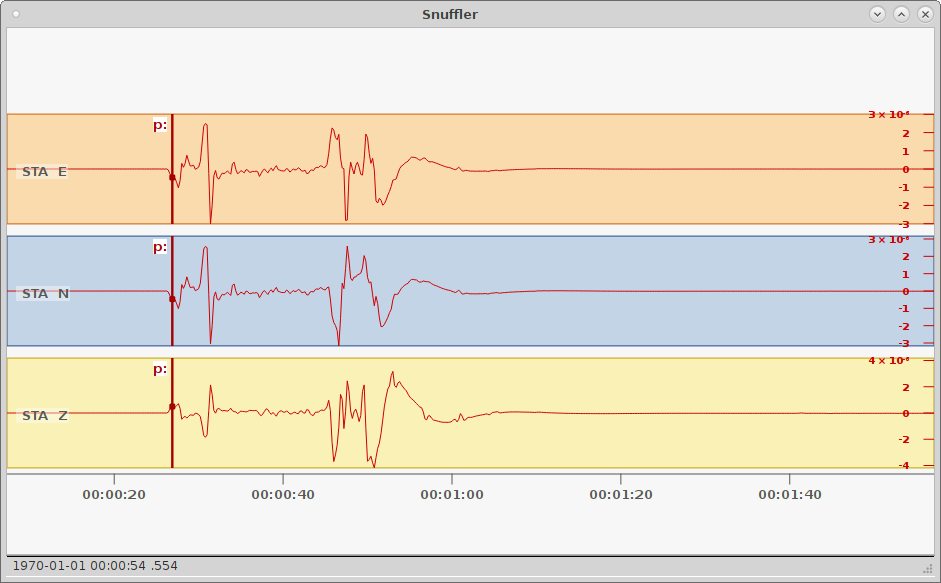
Synthetic seismograms calculated through pyrocko.gf displayed in Snuffler - seismogram browser and workbench. The three traces show the east, north and vertical synthetical displacement stimulated by a double-couple source at 155 km distance.
Calculate spatial surface displacement from a local GF store
In this example we create a RectangularSource and compute the spatial static displacement invoked by that rupture.
We will utilize LocalEngine, StaticTarget and SatelliteTarget.
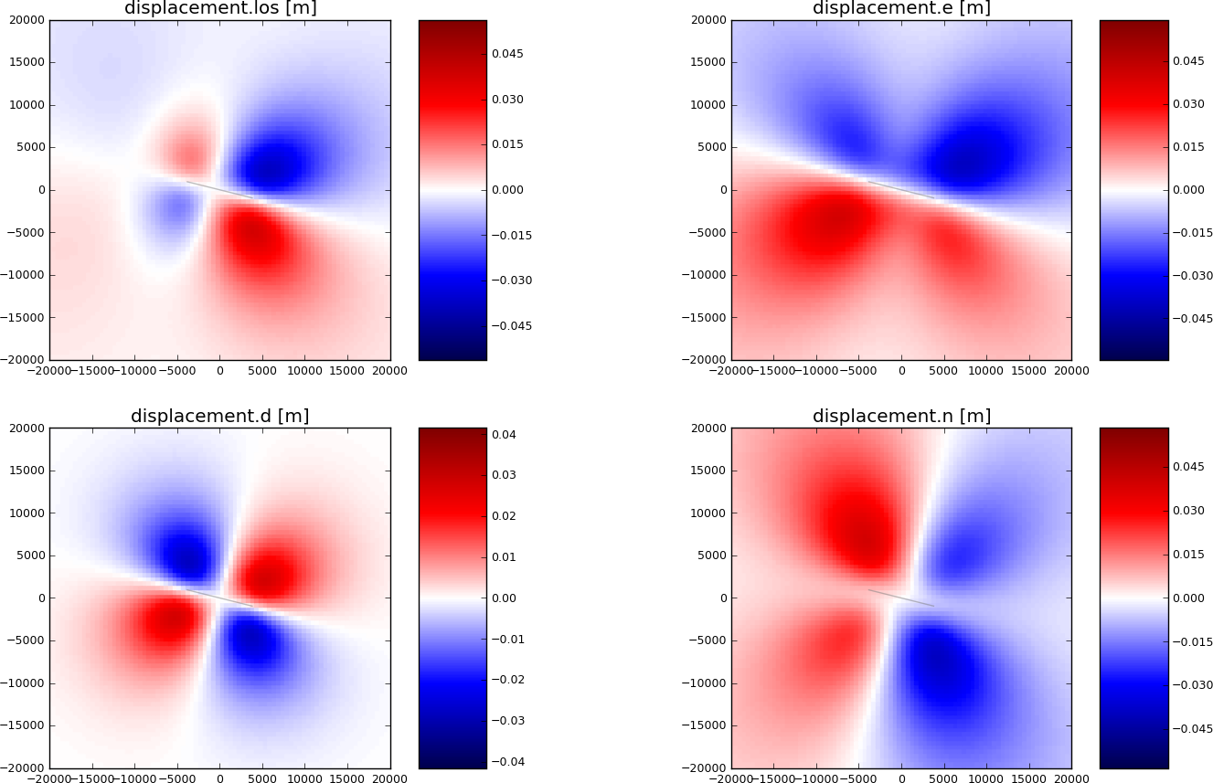
Synthetic surface displacement from a vertical strike-slip fault, with a N104W azimuth, in the Line-of-sight (LOS), east, north and vertical directions. LOS as for Envisat satellite (Look Angle: 23., Heading:-76). Positive motion toward the satellite.
Download gf_forward_example2.py
import os.path
from pyrocko import gf
import numpy as num

# Download a Greens Functions store, programmatically.
store_id = 'gf_abruzzo_nearfield_vmod_Ameri'
if not os.path.exists(store_id):
    gf.ws.download_gf_store(site='kinherd', store_id=store_id)

# Setup the LocalEngine and point it to the fomosto store you just downloaded.
# *store_superdirs* is a list of directories where to look for GF Stores.
engine = gf.LocalEngine(store_superdirs=['.'])

# We define an extended source, in this case a rectangular geometry
# Centroid UTM position is defined relatively to geographical lat, lon position
# Purely lef-lateral strike-slip fault with an N104W azimuth.

km = 1e3  # for convenience

rect_source = gf.RectangularSource(
    lat=0., lon=0.,
    north_shift=0., east_shift=0., depth=6.5*km,
    width=5*km, length=8*km,
    dip=90., rake=0., strike=104.,
    slip=1.)

# We will define a grid of targets
# number in east and north directions, and total
ngrid = 80

# extension from origin in all directions
obs_size = 20.*km
ntargets = ngrid**2

# make regular line vector
norths = num.linspace(-obs_size, obs_size, ngrid)
easts = num.linspace(-obs_size, obs_size, ngrid)

# make regular grid
norths2d = num.repeat(norths, len(easts))
easts2d = num.tile(easts, len(norths))

# We initialize the satellite target and set the line of sight vectors
# direction, example of the Envisat satellite
look = 23.     # angle between the LOS and the vertical
heading = -76  # angle between the azimuth and the east (anti-clock)
theta = num.empty(ntargets)  # vertical LOS from horizontal
theta.fill(num.deg2rad(90. - look))
phi = num.empty(ntargets)  # horizontal LOS from E in anti-clokwise rotation
phi.fill(num.deg2rad(-90-heading))

satellite_target = gf.SatelliteTarget(
    north_shifts=norths2d,
    east_shifts=easts2d,
    tsnapshot=24. * 3600.,  # one day
    interpolation='nearest_neighbor',
    phi=phi,
    theta=theta,
    store_id=store_id)

# The computation is performed by calling process on the engine
result = engine.process(rect_source, [satellite_target])


def plot_static_los_result(result, target=0):
    '''Helper function for plotting the displacement'''

    import matplotlib.pyplot as plt

    # get target coordinates and displacements from results
    N = result.request.targets[target].coords5[:, 2]
    E = result.request.targets[target].coords5[:, 3]
    synth_disp = result.results_list[0][target].result

    # get the component names of displacements
    components = synth_disp.keys()
    fig, _ = plt.subplots(int(len(components)/2), int(len(components)/2))

    vranges = [(synth_disp[k].max(),
                synth_disp[k].min()) for k in components]

    for comp, ax, vrange in zip(components, fig.axes, vranges):

        lmax = num.abs([num.min(vrange), num.max(vrange)]).max()

        # plot displacements at targets as colored points
        cmap = ax.scatter(E, N, c=synth_disp[comp], s=10., marker='s',
                          edgecolor='face', cmap='seismic',
                          vmin=-1.5*lmax, vmax=1.5*lmax)

        ax.set_title(comp+' [m]')
        ax.set_aspect('equal')
        ax.set_xlim(-obs_size, obs_size)
        ax.set_ylim(-obs_size, obs_size)
        # We plot the modeled fault
        n, e = rect_source.outline(cs='xy').T
        ax.fill(e, n, color=(0.5, 0.5, 0.5), alpha=0.5)

        fig.colorbar(cmap, ax=ax, aspect=5)

    plt.show()


plot_static_los_result(result)
Calculate spatial surface displacement and export Kite scenes
We derive InSAR surface deformation targets from Kite scenes. This way we can easily inspect the data and use Kite’s quadtree data sub-sampling and data error variance-covariance estimation calculation.
Download gf_forward_example2_kite.py
import os.path
from kite.scene import Scene, FrameConfig
from pyrocko import gf
import numpy as num

km = 1e3
d2r = num.pi/180.

# Download a Greens Functions store
store_id = 'gf_abruzzo_nearfield_vmod_Ameri'
if not os.path.exists(store_id):
    gf.ws.download_gf_store(site='kinherd', store_id=store_id)

# Setup the modelling LocalEngine
# *store_superdirs* is a list of directories where to look for GF Stores.
engine = gf.LocalEngine(store_superdirs=['.'])

rect_source = gf.RectangularSource(
    # Geographical position [deg]
    lat=0., lon=0.,
    # Relative cartesian offsets [m]
    north_shift=10*km, east_shift=10*km,
    depth=6.5*km,
    # Dimensions of the fault [m]
    width=5*km, length=8*km,
    strike=104., dip=90., rake=0.,
    # Slip in [m]
    slip=1., anchor='top')

# Define the scene's frame
frame = FrameConfig(
    # Lower left geographical reference [deg]
    llLat=0., llLon=0.,
    # Pixel spacing [m] or [degrees]
    spacing='meter', dE=250, dN=250)

# Resolution of the scene
npx_east = 800
npx_north = 800

# 2D arrays for displacement and look vector
displacement = num.empty((npx_east, npx_north))

# Look vectors
# Theta is elevation angle from horizon
theta = num.full_like(displacement, 48.*d2r)
# Phi is azimuth towards the satellite, counter-clockwise from East
phi = num.full_like(displacement, 23.*d2r)

scene = Scene(
    displacement=displacement,
    phi=phi, theta=theta,
    frame=frame)

# Or just load an existing scene!
# scene = Scene.load('my_scene_asc.npy')

satellite_target = gf.KiteSceneTarget(
    scene,
    store_id=store_id)

# Forward model!
result = engine.process(
    rect_source, satellite_target,
    # Use all available cores
    nthreads=0)

kite_scenes = result.kite_scenes()

# Show the synthetic data in spool
# kite_scenes[0].spool()
Calculate forward model of thrust faulting and display wrapped phase
In this example we compare the synthetic unwappred and wrapped LOS displacements caused by a thrust rupture.
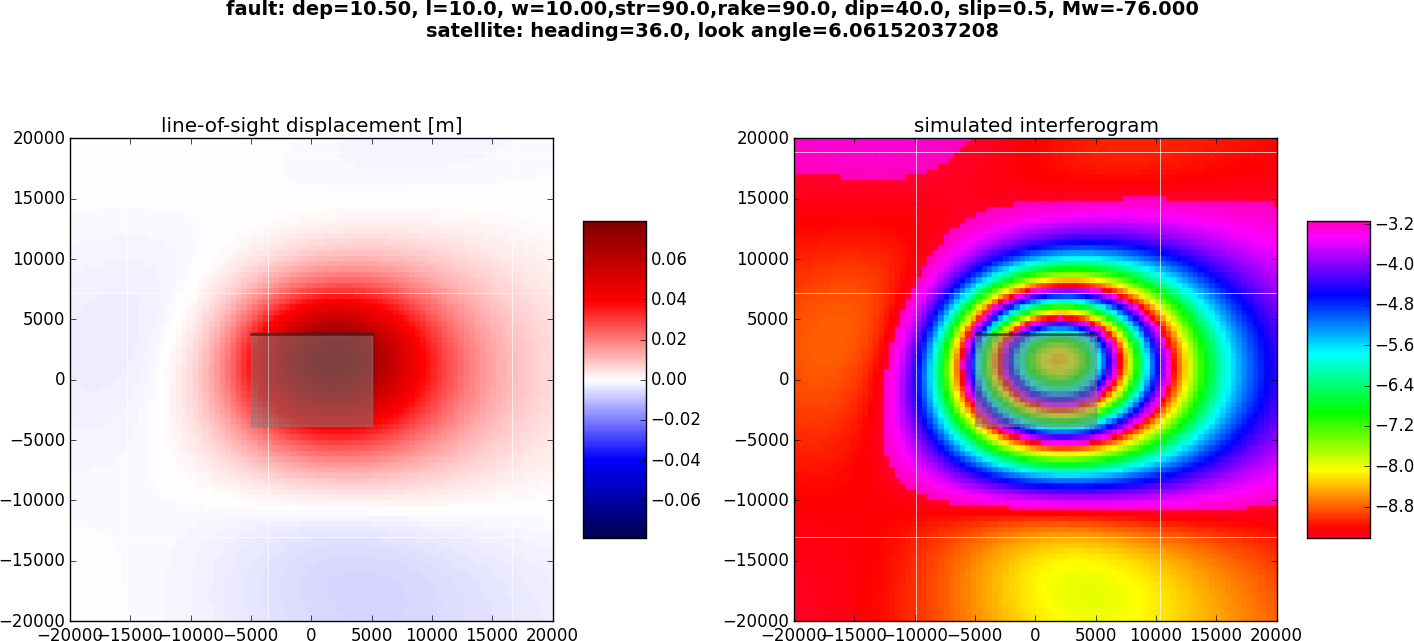
Synthetic LOS displacements from a south-dipping thrust fault. LOS as for Sentinel-1 satellite (Look Angle: 36., Heading:-76). Positive motion toward the satellite. Left: unwrapped phase. Right: Wrapped phase.
Download gf_forward_example3.py
import os.path
import numpy as num
import matplotlib.pyplot as plt
from pyrocko import gf

# Download a Greens Functions store, programmatically.
store_id = 'gf_abruzzo_nearfield_vmod_Ameri'
if not os.path.exists(store_id):
    gf.ws.download_gf_store(site='kinherd', store_id=store_id)

# Ignite the LocalEngine and point it to your fomosto store, e.g. stored on a
# USB stick, which for example has the id 'Abruzzo_Ameri_static_nearfield'
engine = gf.LocalEngine(store_superdirs=['.'])

# We want to reproduce the USGS Solution of an event, e.g.
dep, strike, dip, leng, wid, rake, slip = 10.5, 90., 40., 10., 10., 90., .5

km = 1e3    # distance in kilometer, for convenienve

# We compute the magnitude of the event
potency = leng*km*wid*km*slip
rigidity = 31.5e9
m0 = potency*rigidity
mw = (2./3) * num.log10(m0) - 6.07

# We define an extended rectangular source
thrust = gf.RectangularSource(
    north_shift=0., east_shift=0.,
    depth=dep*km, width=wid*km, length=leng*km,
    dip=dip, rake=rake, strike=strike,
    slip=slip)

# We will define a grid of targets
# number in east and north directions, and total
ngrid = 40
# ngrid = 90  # for better resolution

# extension from origin in all directions
obs_size = 20.*km
ntargets = ngrid**2

# make regular line vector
norths = num.linspace(-obs_size, obs_size, ngrid)
easts = num.linspace(-obs_size, obs_size, ngrid)

# make regular grid
norths2d = num.repeat(norths, len(easts))
easts2d = num.tile(easts, len(norths))

# We initialize the satellite target and set the line of site vectors
# Case example of the Sentinel-1 satellite:
# Heading: -166 (anti-clockwise rotation from east)
# Average Look Angle: 36 (from vertical)
heading = -76.
look = 36.
phi = num.empty(ntargets)    # Horizontal LOS from E in anti-clockwise rotation
theta = num.empty(ntargets)  # Vertical LOS from horizontal
phi.fill(num.deg2rad(-90-heading))
theta.fill(num.deg2rad(90.-look))

satellite_target = gf.SatelliteTarget(
    north_shifts=norths2d,
    east_shifts=easts2d,
    tsnapshot=24.*3600.,    # one day
    interpolation='nearest_neighbor',
    phi=phi,
    theta=theta,
    store_id=store_id)

# The computation is performed by calling 'process' on the engine
result = engine.process(thrust, [satellite_target])

# get synthetic displacements and target coordinates from engine's 'result'
# of the first target (i target=0)
i_target = 0
N = result.request.targets[i_target].coords5[:, 2]
E = result.request.targets[i_target].coords5[:, 3]
synth_disp = result.results_list[0][i_target].result

# we get the fault projection to the surface for plotting
n, e = thrust.outline(cs='xy').T

fig, _ = plt.subplots(1, 2, figsize=(8, 4))
fig.suptitle(
    "fault: dep={:0.2f}, l={}, w={:0.2f},str={},"
    "rake={}, dip={}, slip={}, Mw={:0.3f}\n"
    "satellite: heading={}, look angle={}"
    .format(dep, leng, wid, strike, rake, dip, slip, heading, look, mw),
    fontsize=14,
    fontweight='bold')

# We shift the relative LOS displacements
los = synth_disp['displacement.los']
losrange = [(los.max(), los.min())]
losmax = num.abs([num.min(losrange), num.max(losrange)]).max()

# Plot unwrapped LOS displacements
ax = fig.axes[0]
cmap = ax.scatter(
    E, N, c=los,
    s=10., marker='s',
    edgecolor='face',
    cmap=plt.get_cmap('seismic'),
    vmin=-1.*losmax, vmax=1.*losmax)

ax.set_title('line-of-sight displacement [m]')
ax.set_aspect('equal')
ax.set_xlim(-obs_size, obs_size)
ax.set_ylim(-obs_size, obs_size)
# plot fault outline
ax.fill(e, n, color=(0.5, 0.5, 0.5), alpha=0.5)
# We underline the tip of the thrust
ax.plot(e[:2], n[:2], linewidth=2., color='black', alpha=0.5)

fig.colorbar(cmap, ax=ax, orientation='vertical', aspect=5, shrink=0.5)

# We simulate a C-band interferogram for this source
c_lambda = 0.056
insar_phase = -num.mod(los, c_lambda/2.)/(c_lambda/2.)*2.*num.pi - num.pi

# We plot wrapped phase
ax = fig.axes[1]
cmap = ax.scatter(
    E, N, c=insar_phase,
    s=10., marker='s',
    edgecolor='face',
    cmap=plt.get_cmap('gist_rainbow'))

ax.set_xlim(-obs_size, obs_size)
ax.set_ylim(-obs_size, obs_size)
ax.set_title('simulated interferogram')
ax.set_aspect('equal')

# plot fault outline
ax.fill(e, n, color=(0.5, 0.5, 0.5), alpha=0.5)
# We outline the top edge of the fault with a thick line
ax.plot(e[:2], n[:2], linewidth=2., color='black', alpha=0.5)

fig.colorbar(cmap, orientation='vertical', shrink=0.5, aspect=5)
plt.show()
Combining dislocation sources
In this example we combine two rectangular sources and plot the forward model in profile.
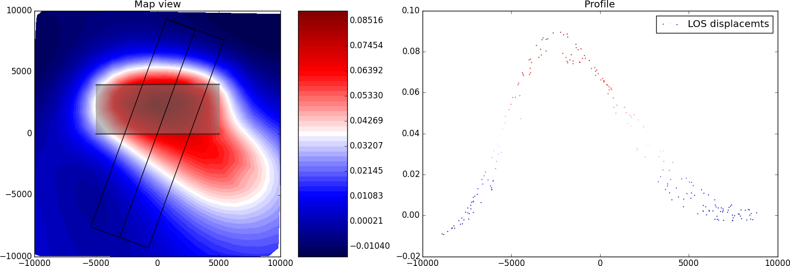
Synthetic LOS displacements from a flower-structure made of one strike-slip fault and one thrust fault. LOS as for Sentinel-1 satellite (Look Angle: 36°, Heading: -76°). Positive motion toward the satellite.
Download gf_forward_example4.py
import os.path
import numpy as num
from pyrocko import gf
from pyrocko.guts import List


class CombiSource(gf.Source):
    '''Composite source model.'''

    discretized_source_class = gf.DiscretizedMTSource

    subsources = List.T(gf.Source.T())

    def __init__(self, subsources=[], **kwargs):

        if subsources:

            lats = num.array(
                [subsource.lat for subsource in subsources], dtype=num.float)
            lons = num.array(
                [subsource.lon for subsource in subsources], dtype=num.float)

            assert num.all(lats == lats[0]) and num.all(lons == lons[0])
            lat, lon = lats[0], lons[0]

            # if not same use:
            # lat, lon = center_latlon(subsources)

            depth = float(num.mean([p.depth for p in subsources]))
            t = float(num.mean([p.time for p in subsources]))
            kwargs.update(time=t, lat=float(lat), lon=float(lon), depth=depth)

        gf.Source.__init__(self, subsources=subsources, **kwargs)

    def get_factor(self):
        return 1.0

    def discretize_basesource(self, store, target=None):
        dsources = []
        t0 = self.subsources[0].time
        for sf in self.subsources:
            assert t0 == sf.time
            ds = sf.discretize_basesource(store, target)
            ds.m6s *= sf.get_factor()
            dsources.append(ds)

        return gf.DiscretizedMTSource.combine(dsources)


# Download a Greens Functions store, programmatically.
store_id = 'gf_abruzzo_nearfield_vmod_Ameri'
if not os.path.exists(store_id):
    gf.ws.download_gf_store(site='kinherd', store_id=store_id)

km = 1e3   # distance in kilometer

# We define a grid for the targets.
left, right, bottom, top = -10*km, 10*km, -10*km, 10*km
ntargets = 1000

# Ignite the LocalEngine and point it to fomosto stores stored on a
# USB stick, for this example we use a static store with id 'static_store'
engine = gf.LocalEngine(store_superdirs=['.'])
store_id = 'gf_abruzzo_nearfield_vmod_Ameri'

# We define two finite sources
# The first one is a purely vertical strike-slip fault
strikeslip = gf.RectangularSource(
    north_shift=0., east_shift=0.,
    depth=6*km, width=4*km, length=10*km,
    dip=90., rake=0., strike=90.,
    slip=1.)

# The second one is a ramp connecting to the root of the strike-slip fault
# ramp north shift (n) and width (w) depend on its dip angle and on
# the strike slip fault width
n, w = 2/num.tan(num.deg2rad(45.)), 2.*(2./(num.sin(num.deg2rad(45.))))
thrust = gf.RectangularSource(
    north_shift=n*km, east_shift=0.,
    depth=6*km, width=w*km, length=10*km,
    dip=45., rake=90., strike=90.,
    slip=0.5)

# We initialize the satellite target and set the line of site vectors
# Case example of the Sentinel-1 satellite:
# Heading: -166 (anti clockwise rotation from east)
# Average Look Angle: 36 (from vertical)
heading = -76
look = 36.
phi = num.empty(ntargets)    # Horizontal LOS from E in anti-clockwise rotation
theta = num.empty(ntargets)  # Vertical LOS from horizontal
phi.fill(num.deg2rad(-90. - heading))
theta.fill(num.deg2rad(90. - look))

satellite_target = gf.SatelliteTarget(
    north_shifts=num.random.uniform(bottom, top, ntargets),
    east_shifts=num.random.uniform(left, right, ntargets),
    tsnapshot=24.*3600.,
    interpolation='nearest_neighbor',
    phi=phi,
    theta=theta,
    store_id=store_id)

# We combine the two sources here
patches = [strikeslip, thrust]
sources = CombiSource(subsources=patches)

# The computation is performed by calling process on the engine
result = engine.process(sources, [satellite_target])


def plot_static_los_profile(result, strike, l, w, x0, y0):  # noqa
    import matplotlib.pyplot as plt
    import matplotlib.cm as cm
    import matplotlib.colors as mcolors
    fig, _ = plt.subplots(1, 2, figsize=(8, 4))

    # strike,l,w,x0,y0: strike, length, width, x, and y position
    # of the profile
    strike = num.deg2rad(strike)
    # We define the parallel and perpendicular vectors to the profile
    s = [num.sin(strike), num.cos(strike)]
    n = [num.cos(strike), -num.sin(strike)]

    # We define the boundaries of the profile
    ypmax, ypmin = l/2, -l/2
    xpmax, xpmin = w/2, -w/2

    # We define the corners of the profile
    xpro, ypro = num.zeros((7)), num.zeros((7))
    xpro[:] = x0-w/2*s[0]-l/2*n[0], x0+w/2*s[0]-l/2*n[0], \
        x0+w/2*s[0]+l/2*n[0], x0-w/2*s[0]+l/2*n[0], x0-w/2*s[0]-l/2*n[0], \
        x0-l/2*n[0], x0+l/2*n[0]

    ypro[:] = y0-w/2*s[1]-l/2*n[1], y0+w/2*s[1]-l/2*n[1], \
        y0+w/2*s[1]+l/2*n[1], y0-w/2*s[1]+l/2*n[1], y0-w/2*s[1]-l/2*n[1], \
        y0-l/2*n[1], y0+l/2*n[1]

    # We get the forward model from the engine
    N = result.request.targets[0].coords5[:, 2]
    E = result.request.targets[0].coords5[:, 3]
    result = result.results_list[0][0].result

    # We first plot the surface displacements in map view
    ax = fig.axes[0]
    los = result['displacement.los']
    levels = num.linspace(los.min(), los.max(), 50)

    cmap = ax.tricontourf(E, N, los, cmap=plt.get_cmap('seismic'),
                          levels=levels)

    for sourcess in patches:
        fn, fe = sourcess.outline(cs='xy').T
        ax.fill(fe, fn, color=(0.5, 0.5, 0.5), alpha=0.5)
        ax.plot(fe[:2], fn[:2], linewidth=2., color='black', alpha=0.5)

    # We plot the limits of the profile in map view
    ax.plot(xpro[:], ypro[:], color='black', lw=1.)
    # plot colorbar
    fig.colorbar(cmap, ax=ax, orientation='vertical', aspect=5)
    ax.set_title('Map view')
    ax.set_aspect('equal')

    # We plot displacements in profile
    ax = fig.axes[1]
    # We compute the perpendicular and parallel components in the profile basis
    yp = (E-x0)*n[0]+(N-y0)*n[1]
    xp = (E-x0)*s[0]+(N-y0)*s[1]
    los = result['displacement.los']

    # We select data encompassing the profile
    index = num.nonzero(
        (xp > xpmax) | (xp < xpmin) | (yp > ypmax) | (yp < ypmin))

    ypp, losp = num.delete(yp, index), \
        num.delete(los, index)

    # We associate the same color scale to the scatter plot
    norm = mcolors.Normalize(vmin=los.min(), vmax=los.max())
    m = cm.ScalarMappable(norm=norm, cmap=plt.get_cmap('seismic'))
    facelos = m.to_rgba(losp)
    ax.scatter(
        ypp, losp,
        s=0.3, marker='o', color=facelos, label='LOS displacements')

    ax.legend(loc='best')
    ax.set_title('Profile')

    plt.show()


plot_static_los_profile(result, 110., 18*km, 5*km, 0., 0.)
Modelling viscoelastic static displacement
In this advanced example we leverage the viscoelastic forward modelling capabilities of the psgrn_pscmp backend.
Viscoelastic static GF store forward-modeling the transient effects of a deep dislocation source, mimicking a transform plate boundary. Together with a shallow seismic source. The cross denotes the tracked pixel location. (Top) Displacement of the tracked pixel in time.
The static store has to be setup with Burger material describing the viscoelastic properties of the medium, see this config for the fomosto store:
Note
Static stores define the sampling rate in Hz.
sampling_rate: 1.157e-06 Hz is a sampling rate of 10 days!
--- !pf.ConfigTypeA
id: static_t
modelling_code_id: psgrn_pscmp.2008a
regions: []
references: []
earthmodel_1d: |2
      0.             2.5            1.2            2.1           50.            50.
      1.             2.5            1.2            2.1           50.            50.
      1.             6.2            3.6            2.8          600.           400.
     17.             6.2            3.6            2.8          600.           400.
     17.             6.6            3.7            2.9         1432.           600.
     32.             6.6            3.7            2.9         1432.           600.
     32.             7.3            4.             3.1         1499.           600.            1e30            1e20           1.
     41.             7.3            4.             3.1         1499.           600.            1e30            1e20           1.
  mantle
     41.             8.2            4.7            3.4         1370.           600.            1e19            5e17           1.
     91.             8.2            4.7            3.4         1370.           600.            1e19            5e17           1.
sample_rate: 1.1574074074074074e-06
component_scheme: elastic10
tabulated_phases: []
ncomponents: 10
receiver_depth: 0.0
source_depth_min: 0.0
source_depth_max: 40000.0
source_depth_delta: 500.0
distance_min: 0.0
distance_max: 150000.0
distance_delta: 1000.0
In the extra/psgrn_pscmp configruation file we have to define the timespan from tmin_days to tmax_days, covered by the sampling_rate (see above)
--- !pf.PsGrnPsCmpConfig
tmin_days: 0.0
tmax_days: 600.0
gf_outdir: psgrn_functions
psgrn_config: !pf.PsGrnConfig
  version: 2008a
  sampling_interval: 1.0
  gf_depth_spacing: -1.0
  gf_distance_spacing: -1.0
  observation_depth: 0.0
pscmp_config: !pf.PsCmpConfig
  version: 2008a
  observation: !pf.PsCmpScatter {}
  rectangular_fault_size_factor: 1.0
  rectangular_source_patches: []
Download gf_forward_viscoelastic.py
'''
An advanced example requiring a viscoelastic static store.
See https://pyrocko.org for detailed instructions.
'''
import logging
import os.path as op
import matplotlib.pyplot as plt
from matplotlib.animation import FuncAnimation
from matplotlib.ticker import FuncFormatter

import numpy as num
from pyrocko import gf

logging.basicConfig(level=logging.INFO)
logger = logging.getLogger('static-viscoelastic')

km = 1e3
d2r = num.pi/180.
store_id = 'static_t'

day = 3600*24

engine = gf.LocalEngine(store_superdirs=['.'])

ngrid = 100

extent = (-75*km, 75*km)
dpx = abs((extent[0] - extent[1]) / ngrid)

easts = num.linspace(*extent, ngrid)
norths = num.linspace(*extent, ngrid)
east_shifts = num.tile(easts, ngrid)
north_shifts = num.repeat(norths, ngrid)

look = 23.
heading = -76.  # descending
npx = int(ngrid**2)

tmax = 1000*day
t_eq = 200*day
nsteps = 200

dt = tmax / nsteps

satellite_target = gf.SatelliteTarget(
    east_shifts=east_shifts,
    north_shifts=north_shifts,
    phi=num.full(npx, d2r*(90.-look)),
    theta=num.full(npx, d2r*(-90.-heading)),
    interpolation='nearest_neighbor')

creep_source = gf.RectangularSource(
    lat=0., lon=0.,
    north_shift=3*km, east_shift=0.,
    depth=25*km,
    width=15*km, length=80*km,
    strike=100., dip=90., rake=0.,
    slip=0.08, anchor='top',
    decimation_factor=4)

coseismic_sources = gf.RectangularSource(
    lat=0., lon=0.,
    north_shift=3*km, east_shift=0.,
    depth=15*km,
    width=10*km, length=60*km,
    strike=100., dip=90., rake=0.,
    slip=.5, anchor='top',
    decimation_factor=4,
    time=t_eq)

targets = []
for istep in range(nsteps):
    satellite_target = gf.SatelliteTarget(
        east_shifts=east_shifts,
        north_shifts=north_shifts,
        phi=num.full(npx, d2r*(90.-look)),
        theta=num.full(npx, d2r*(-90.-heading)),
        interpolation='nearest_neighbor',
        tsnapshot=dt*istep)
    targets.append(satellite_target)


def get_displacement(sources, targets, component='los'):
    result = engine.process(
        sources, targets,
        nthreads=0)

    static_results = result.static_results()
    nres = len(static_results)

    res_arr = num.empty((nres, ngrid, ngrid))

    for ires, res in enumerate(static_results):
        res_arr[ires] = res.result['displacement.%s' % component]\
            .reshape(ngrid, ngrid)
    return res_arr


component = 'los'
fn = 'displacement_%s' % component

# Use cached displacements
if not op.exists('%s.npy' % fn):
    logger.info('Calculating scenario for %s.npy ...', fn)
    displacement_creep = get_displacement(
        creep_source, satellite_target, component)[0]
    displacement_creep /= 365.

    displacement = get_displacement(coseismic_sources, targets, component)

    for istep in range(nsteps):
        displacement[istep] += displacement_creep * (dt / day) * istep

    num.save(fn, displacement)
else:
    logger.info('Loading scenario data from %s.npy ...', fn)
    displacement = num.load('%s.npy' % fn)

if False:
    fig = plt.figure()
    ax = fig.gca()

    for ipx in range(ngrid)[::10]:
        for ipy in range(ngrid)[::10]:
            ax.plot(displacement[:, ipx, ipy], alpha=.3, color='k')

    plt.show()


sample_point = (-20.*km, -27.*km)
sample_idx = (int(sample_point[0] / dpx), int(sample_point[1] / dpx))

fig, (ax_time, ax_u) = plt.subplots(
    2, 1, gridspec_kw={'height_ratios': [1, 4]})
fig.set_size_inches(10, 8)
ax_u = fig.gca()

vrange = num.abs(displacement).max()
colormesh = ax_u.pcolormesh(
    easts, norths, displacement[80],
    cmap='seismic', vmin=-vrange, vmax=vrange, shading='gouraud',
    animated=True)

smpl_point = ax_u.scatter(
    *sample_point, marker='x', color='black', s=30, zorder=30)

time_label = ax_u.text(.95, .05, '0 days', ha='right', va='bottom',
                       alpha=.5, transform=ax_u.transAxes, zorder=20)

# cbar = fig.colorbar(img)
# cbar.set_label('Displacment %s [m]', )

ax_u.set_xlabel('Easting [km]')
ax_u.set_ylabel('Northing [km]')

km_formatter = FuncFormatter(lambda x, pos: x / km)
ax_u.xaxis.set_major_formatter(km_formatter)
ax_u.yaxis.set_major_formatter(km_formatter)

ax_time.set_title('%s Displacement' % component.upper())
urange = (displacement[:, sample_idx[0], sample_idx[1]].min() * 1.05,
          displacement[:, sample_idx[0], sample_idx[1]].max() * 1.05)
ut = ax_time.plot([], [], color='black')[0]
ax_time.axvline(x=t_eq + dt, linestyle='--', color='red', alpha=.5)

day_formatter = FuncFormatter(lambda x, pos: int(x / day))
ax_time.xaxis.set_major_formatter(day_formatter)
ax_time.set_xlim(0., tmax)
ax_time.set_ylim(*urange)

ax_time.set_xlabel('Days')
ax_time.set_ylabel('Displacement [m]')
ax_time.grid(alpha=.3)


def animation_update(frame):
    colormesh.set_array(displacement[frame].ravel())
    time_label.set_text('%d days' % int(frame * (dt / day)))

    ut.set_xdata(num.arange(frame) * dt)
    ut.set_ydata(displacement[:frame, sample_idx[0], sample_idx[1]])

    return colormesh, smpl_point, time_label, ut


ani = FuncAnimation(
    fig, animation_update, frames=nsteps, interval=30, blit=True)
# plt.show()

logger.info('Saving animation...')
ani.save('viscoelastic-response.mp4', writer='ffmpeg')
Creating a custom Source Time Function (STF)
Basic example how to create a custom STF class, creating a linearly decreasing ramp excitation.
Download gf_custom_stf.py
from pyrocko.gf import STF
from pyrocko.guts import Float
import numpy as num


class LinearRampSTF(STF):
    '''Linearly decreasing ramp from maximum amplitude to zero.'''

    duration = Float.T(
        default=0.0,
        help='baseline of the ramp')

    anchor = Float.T(
        default=0.0,
        help='anchor point with respect to source-time: ('
             '-1.0: left -> source duration [0, T] ~ hypocenter time, '
             ' 0.0: center -> source duration [-T/2, T/2] ~ centroid time, '
             '+1.0: right -> source duration [-T, 0] ~ rupture end time)')

    def discretize_t(self, deltat, tref):
        # method returns discrete times and the respective amplitudes
        tmin_stf = tref - self.duration * (self.anchor + 1.) * 0.5
        tmax_stf = tref + self.duration * (1. - self.anchor) * 0.5
        tmin = round(tmin_stf / deltat) * deltat
        tmax = round(tmax_stf / deltat) * deltat
        nt = int(round((tmax - tmin) / deltat)) + 1
        times = num.linspace(tmin, tmax, nt)
        if nt > 1:
            amplitudes = num.linspace(1., 0., nt)
            amplitudes /= num.sum(amplitudes)  # normalise to keep moment
        else:
            amplitudes = num.ones(1)

        return times, amplitudes

    def base_key(self):
        # method returns STF name and the values
        return (self.__class__.__name__, self.duration, self.anchor)