Pyrocko Workshop @dgg2021

By Team Pyrocko

What is Pyrocko?

• Software building blocks
• Tools to make seismologists happy

• Tight integration
• Common look-and-feel

Workflows

Functionality: Data Sources

• IO modules for seismological data formats
• Clients for FDSN and online catalogs
• Datalogger and real-time data support
• Datasets: velocity profiles, earth models, topography, volcanoes, geonames, gshhg

Functionality: Processing

• Simple data model for station meta-data, seismic events, waveform markers
• Waveform data processing
• Static displacements handling
• Instrument response representations and evaluation
• Waveform archive and metadata indexing and database
• Parallel and GPU waveform stacking for migration and array processing

Functionality: Modelling

• Travel-time and ray-path computations
• Fast hierarchical travel-time interpolator
• Pre-computed Green's functions
• Synthetic seismogram generator
• Fast 2D/3D FMM eikonal solver
• Okada modelling
• Boundary element modelling
• Rupture models

Functionality: miscellaneous

• Moment tensor utilities and plotting
• Plotting utilities, Hudson plots, maps, GMT interface, seismic rays
• Geodesic helper functions
• High sampling rate support (micro-acoustics)
• YAML data serialization for almost all internal objects
• ObsPy compatibility
• Tons of utility functions

Functionality: Front-End Tools

• Waveform viewer, picker, workbench, with lots of plugins
• Travel-times and ray paths
• Green's function computation front end
• Data format conversion
• Random synthetic scenario generator for events, waveforms, GNSS, InSAR

Pyrocko is hard open source

License: GPLv3 = strong copyleft. Why?

• Support reproducible, transparent research.
• Natural hazards are public concern.
• Our contracts are paid from public money.

Contribute

Join us at the friendly Pyrocko Hive!

Pyrocko Snuffler

Snuffle through a pile of seismic data.

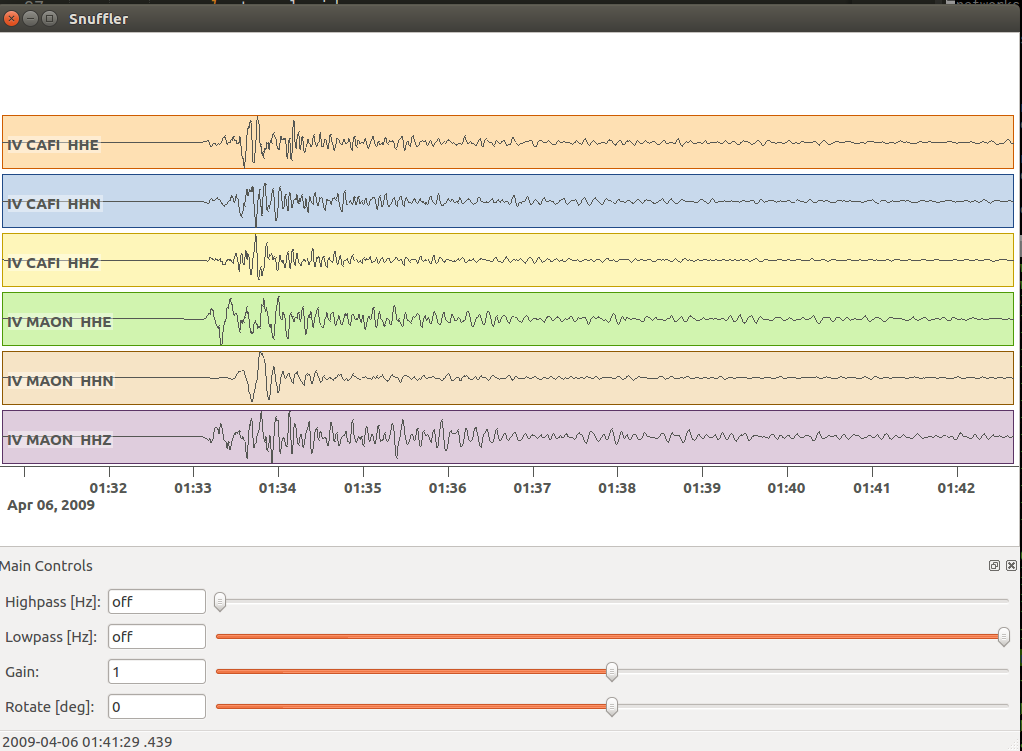
Lets start to snuffle - 2009 M_w 6.3 L'Aquila

generated using pyrocko.plot.automap

Get data

# Download waveforms, event and station data
url_base=https://data.pyrocko.org/examples/laquila_small
wget $url_base/traces.mseed
wget $url_base/stations.txt
wget $url_base/laquila.pf

# open traces.mseed in snuffler
snuffler traces.mseed
                    

Main controls

For help press ?

Zoom

Zoom

Zoom

Navigate

or press b (backwards), space (forward)

Navigate

Scaling

Quick search

Quick search

Quick search

Filter

Filter

Filter

The main menu

reachable via right mouse click

Load station meta data

# Start Snuffler with station information
snuffler traces.mseed --stations=stations.txt  # or
snuffler traces.mseed --stationxml=stations.xml
                        

or ...

Load station meta data

Load station meta data

Load station meta data

Load event data

# Start Snuffler with event information
snuffler traces.mseed --event=laquila.pf
                        

or ...

Load event data

Load event data

Load event data

Load event data

Load event data

Load event data

Map view

Map view

Map view

Phase arrivals

Phase arrivals

Phase arrivals

Snuffler - many more ways of looking at data

Extend Snuffler with Plugins (Snufflings)

Pyrocko Scripts

Simple Python scripting for seismic data analysis with Pyrocko.

From catalog search to seismic data analysis

L'Aquila 2009-04-06, Mw 6.3

Catalog search

import os
from pyrocko import model, util, trace, pile
from pyrocko.client import catalog, fdsn

tmin = util.str_to_time('2009-04-06 01:00:00')
tmax = util.str_to_time('2009-04-07 02:00:00')

min_mag = 4.5  # minimum magnitude
latmin = 40.0  # restrict search for Central Italy
latmax = 44.0
lonmin = 10.0
lonmax = 15.0


                        

Catalog search

geofon = catalog.Geofon()

events = geofon.get_events(
    time_range=(tmin, tmax),
    magmin=min_mag,
    latmin=latmin,
    latmax=latmax,
    lonmin=lonmin,
    lonmax=lonmax)

model.dump_events(events, 'laquila.pf')
                        

Catalog search

''' Output:
name = gfz2009gtfx
time = 2009-04-06 23:15:40.200
latitude = 42.4
longitude = 13.4
magnitude = 4.7
moment = 1.25893e+16
magnitude_type = M
depth = 5000
region = Central Italy
catalog = GEOFON
tags = geofon_status:A, geofon_category:big
--------------------------------------------
name = gfz2009grqp
time = 2009-04-06 02:37:08.000
latitude = 42.4
longitude = 13.3
magnitude = 4.8
moment = 1.77828e+16
magnitude_type = M
depth = 5000
region = Central Italy
catalog = GEOFON
tags = geofon_status:A, geofon_category:big
--------------------------------------------
name = gfz2009groy
time = 2009-04-06 01:32:42.200
latitude = 42.4
longitude = 13.3
magnitude = 6.2
moment = 2.23872e+18
magnitude_type = M
depth = 10000
region = Central Italy
catalog = GEOFON
tags = geofon_status:M, geofon_category:xxl
--------------------------------------------
'''


                        

FDSN download

outdir = 'data'
util.ensuredir(outdir)

for event in events:
    evtmin = event.time - 120
    evtmax = event.time + 600

    # select stations by their NSLC id and wildcards
    selection = [
        ('IV', 'CAFI', '*', 'HH*', evtmin, evtmax),
        ('IV', 'MAON', '*', 'HH*', evtmin, evtmax),
    ]

    # setup a waveform data request
    request_waveform = fdsn.dataselect(site='ingv',
                            selection=selection)

    # write the incoming data stream
    outpath = os.path.join(outdir, 'traces_%s.mseed' % event.name)
    with open(outpath, 'wb') as file:
        file.write(request_waveform.read())


                        

FDSN download

outdir = 'data'
util.ensuredir(outdir)

for event in events:
    evtmin = event.time - 120
    evtmax = event.time + 600

    # select stations by their NSLC id and wildcards
    selection = [
        ('IV', 'CAFI', '*', 'HH*', evtmin, evtmax),
        ('IV', 'MAON', '*', 'HH*', evtmin, evtmax),
    ]

    # setup a waveform data request
    request_waveform = fdsn.dataselect(site='ingv',
                            selection=selection)

    # write the incoming data stream
    outpath = os.path.join(outdir,
                           'traces_%s.mseed' % event.name)

    with open(outpath, 'wb') as file:
        file.write(request_waveform.read())


                        

FDSN download

outdir = 'data'
util.ensuredir(outdir)

for event in events:
    evtmin = event.time - 120
    evtmax = event.time + 600

    # select stations by their NSLC id and wildcards
    selection = [
        ('IV', 'CAFI', '*', 'HH*', evtmin, evtmax),
        ('IV', 'MAON', '*', 'HH*', evtmin, evtmax),
    ]

    # setup a waveform data request
    request_waveform = fdsn.dataselect(site='ingv',
                            selection=selection)

    # write the incoming data stream
    outpath = os.path.join(outdir,
                           'traces_%s.mseed' % event.name)

    with open(outpath, 'wb') as file:
        file.write(request_waveform.read())


                        

FDSN download

# request station meta data for full time span:
selection = [
    ('IV', 'CAFI', '*', 'HH*', tmin, tmax),
    ('IV', 'MAON', '*', 'HH*', tmin, tmax),
]

sxml = fdsn.station(
    site='ingv', selection=selection, level='response')

                        

FDSN download

# request station meta data for full time span:
selection = [
    ('IV', 'CAFI', '*', 'HH*', tmin, tmax),
    ('IV', 'MAON', '*', 'HH*', tmin, tmax),
]

sxml = fdsn.station(
    site='ingv', selection=selection, level='response')

                        

The pile - Waveform archive lookup, data loading and caching infrastructure.

# Browse through all files in a directory
# (without loading data to memory)

p = pile.make_pile(paths=outdir)
print(p)

                        

The pile - Waveform archive lookup, data loading and caching infrastructure.

Restitution, Rotation, Filter

# Iterate over data in pile to restitute and filter
# Select to only iterate over data of station CAFI

displacement = []
for traces in p.chopper(tmin=tmin, tmax=tmax,
        trace_selector=lambda tr: tr.nslc_id[1] == 'CAFI'):

    for tr in traces:
        polezero_response = sxml.get_pyrocko_response(
            nslc=tr.nslc_id,
            timespan=(tr.tmin, tr.tmax),
            fake_input_units='M')
            # *fake_input_units*: required for consistent responses
            # throughout entire data set

        # deconvolve transfer function
        restituted = tr.transfer(
            tfade=2.,
            freqlimits=(0.01, 0.1, 1., 2.),
            transfer_function=polezero_response,
            invert=True)

        # apply a lowpass filter
        tr.lowpass(4, 0.3)

        displacement.append(restituted)


                        

Restitution, Rotation, Filter

# Iterate over data in pile to restitute and filter
# Select to only iterate over data of station CAFI

displacement = []
for traces in p.chopper(tmin=tmin, tmax=tmax,
        trace_selector=lambda tr: tr.nslc_id[1] == 'CAFI'):

    for tr in traces:
        polezero_response = sxml.get_pyrocko_response(
            nslc=tr.nslc_id,
            timespan=(tr.tmin, tr.tmax),
            fake_input_units='M')
            # *fake_input_units*: required for consistent responses
            # throughout entire data set

        # deconvolve transfer function
        tr_restituted = tr.transfer(
            tfade=2.,
            freqlimits=(0.01, 0.1, 1., 2.),
            transfer_function=polezero_response,
            invert=True)

        # apply a lowpass filter
        tr_restituted.lowpass(4, 0.3)

        displacement.append(tr_restituted)


                        

Restitution, Rotation, Filter

# Iterate over data in pile to restitute and filter
# Select to only iterate over data of station CAFI

displacement = []
for traces in p.chopper(tmin=tmin, tmax=tmax,
        trace_selector=lambda tr: tr.nslc_id[1] == 'CAFI'):

    for tr in traces:
        polezero_response = sxml.get_pyrocko_response(
            nslc=tr.nslc_id,
            timespan=(tr.tmin, tr.tmax),
            fake_input_units='M')
            # *fake_input_units*: required for consistent responses
            # throughout entire data set

        # deconvolve transfer function
        tr_restituted = tr.transfer(
            tfade=2.,
            freqlimits=(0.01, 0.1, 1., 2.),
            transfer_function=polezero_response,
            invert=True)

        # apply a lowpass filter
        tr_restituted.lowpass(4, 0.3)

        displacement.append(tr_restituted)


                        

Restitution, Rotation, Filter

# Iterate over data in pile to restitute and filter
# Select to only iterate over data of station CAFI

displacement = []
for traces in p.chopper(tmin=tmin, tmax=tmax,
    trace_selector=lambda tr: tr.nslc_id[1] == 'CAFI'):

    for tr in traces:
        polezero_response = sxml.get_pyrocko_response(
            nslc=tr.nslc_id,
            timespan=(tr.tmin, tr.tmax),
            fake_input_units='M')
            # *fake_input_units*: required for consistent responses
            # throughout entire data set

        # deconvolve transfer function
        tr_restituted = tr.transfer(
            tfade=2.,
            freqlimits=(0.01, 0.1, 1., 2.),
            transfer_function=polezero_response,
            invert=True)

        # apply a lowpass filter
        tr_restituted.lowpass(4, 0.3)

        displacement.append(tr_restituted)


                        

Visualization

trace.snuffle(displacement)

                        

Full script

import os
from pyrocko import model, util, trace, pile
from pyrocko.client import catalog, fdsn


# Search for L'Aquila earthquake and aftershocks on first day
# in Geofon catalog:

tmin = util.str_to_time('2009-04-06 01:00:00')
tmax = util.str_to_time('2009-04-07 02:00:00')

min_mag = 4.5  # minimum magnitude
latmin = 40.0  # restrict search for Central Italy
latmax = 44.0
lonmin = 10.0
lonmax = 15.0

geofon = catalog.Geofon()
events = geofon.get_events(time_range=(tmin, tmax),
                           magmin=min_mag,
                           latmin=latmin,
                           latmax=latmax,
                           lonmin=lonmin,
                           lonmax=lonmax)

model.dump_events(events, 'laquila.pf')

''' Output:
name = gfz2009gtfx
time = 2009-04-06 23:15:40.200
latitude = 42.4
longitude = 13.4
magnitude = 4.7
moment = 1.25893e+16
magnitude_type = M
depth = 5000
region = Central Italy
catalog = GEOFON
tags = geofon_status:A, geofon_category:big
--------------------------------------------
name = gfz2009grqp
time = 2009-04-06 02:37:08.000
latitude = 42.4
longitude = 13.3
magnitude = 4.8
moment = 1.77828e+16
magnitude_type = M
depth = 5000
region = Central Italy
catalog = GEOFON
tags = geofon_status:A, geofon_category:big
--------------------------------------------
name = gfz2009groy
time = 2009-04-06 01:32:42.200
latitude = 42.4
longitude = 13.3
magnitude = 6.2
moment = 2.23872e+18
magnitude_type = M
depth = 10000
region = Central Italy
catalog = GEOFON
tags = geofon_status:M, geofon_category:xxl
--------------------------------------------
'''


# Download seismic waveform data from FDSN

# Load earthquake information
events = model.load_events('laquila.pf')

outdir = 'data'
util.ensuredir(outdir)

for event in events:
    evtmin = event.time - 120
    evtmax = event.time + 600

    # select stations by their NSLC id and wildcards
    selection = [
        ('IV', 'CAFI', '*', 'HH*', evtmin, evtmax),
        ('IV', 'MAON', '*', 'HH*', evtmin, evtmax),
    ]

    # setup a waveform data request
    request_waveform = fdsn.dataselect(site='ingv', selection=selection)

    # write the incoming data stream
    outpath = os.path.join(outdir, 'traces_%s.mseed' % event.name)
    with open(outpath, 'wb') as file:
        file.write(request_waveform.read())


# request station meta data for full time span:
selection = [
    ('IV', 'CAFI', '*', 'HH*', tmin, tmax),
    ('IV', 'MAON', '*', 'HH*', tmin, tmax),
]

sxml = fdsn.station(
    site='ingv', selection=selection, level='response')


# browse through all files in a directory
# (without loading data to memory)
p = pile.make_pile(paths=outdir)
print(p)


# iterate over data in pile to restitute and filter
# select to only iterate over data of station CAFI
displacement = []
for traces in p.chopper(tmin=tmin, tmax=tmax,
                        trace_selector=lambda tr: tr.nslc_id[1] == 'CAFI'):
    for tr in traces:
        polezero_response = sxml.get_pyrocko_response(
            nslc=tr.nslc_id,
            timespan=(tr.tmin, tr.tmax),
            fake_input_units='M')
            # *fake_input_units*: required for consistent responses
            # throughout entire data set

        # deconvolve transfer function
        tr_restituted = tr.transfer(
            tfade=2.,
            freqlimits=(0.01, 0.1, 1., 2.),
            transfer_function=polezero_response,
            invert=True)

        # apply a lowpass filter
        tr_restituted.lowpass(4, 0.3)

        displacement.append(tr_restituted)

# Inspect waveforms using Snuffler
trace.snuffle(displacement)


                        

Pyrocko plotting examples

Pyrocko-GF

Geophysical forward modelling with pre-calculated Green's functions.

Pyrocko-GF at a Glance

• Flexible framework to store and work with pre-calculated Green's functions
• Supports the simulation of various dislocation sources
• Supports both dynamic and static modelling applications

                                    from pyrocko import gf
                                

Green's Function (GF) Stores

                                # Run this in your terminal
                                fomosto download kinherd global_2s_dgg
                            

Source Models

Example: Point Sources

Double Couple

                                    dc_source = gf.DCSource(
                                        lat=54.0, lon=7.0, depth=5.0e3,
                                        strike=21.0, dip=63.0, rake=45.0,
                                        magnitude=4.0)
                                

Moment Tensor

                                    # NOTE: convension used by Pyrocko is
                                    # north-east-down (NED) coordinate system

                                    mt_source = gf.MTSource(
                                        lat=20.0, lon=58.0, depth=8.0e3,
                                        mnn=-3.87e+26, mee=2.13e+26, mdd=1.74e+26,
                                        mne=-2.74e+26, mnd=-0.53e+26, med=1.06e+26)
                                

Example: Finite Sources

Rectangular Fault

                                    KM2M = 1.0e3

                                    rect_source = gf.RectangularSource(
                                        lat=31.0, lon=44.0, depth=5*KM2M,
                                        strike=104.0, dip=90.0, rake=5.0,
                                        length=8*KM2M, width=3*KM2M,
                                        slip=1.3)
                                

Source Time Functions (STF)

Temporal evolution of the seismic moment release

Example: STF

Boxcar

                                    # Times relative to centroid time
                                    stf1 = gf.BoxcarSTF(
                                        duration=4.0, anchor=0.0)
                                

Triangular

                                    # Times relative to hypocentre time
                                    stf2 = gf.TriangularSTF(
                                        duration=4.0, anchor=-1.0)
                                

Half Sinusoid

                                    # Times relative to rupture end-time
                                    stf3 = gf.HalfSinusoidSTF(
                                        duration=4.0, anchor=+1.0)
                                

Modelling Targets (Receivers)

Data structures for holding observer properties

Example: Waveform Targets

A Seismometer

                            waveform_targets = []

                            for channel_code in ('BHE', 'BHN', 'BHZ'):
                                target = gf.Target(
                                    lat=48.3301, lon=8.3296, elevation=638.0,
                                    codes=('II', 'BFO', '00', channel_code),
                                    quantity='velocity',
                                    store_id='global_2s_dgg')

                                waveform_targets.append(target)
                        

Example: Static Displacement Targets

A Campaign GPS Site

                                    import numpy as np

                                    KM2M = 1.0e3

                                    norths = np.linspace(-20*KM2M, 20*KM2M, 100)
                                    easts = np.linspace(-20*KM2M, 20*KM2M, 100)
                                    north_shifts, east_shifts = np.meshgrid(
                                        norths, easts)

                                    gnss_target = gf.GNSSCampaignTarget(
                                        north_shifts=north_shifts,
                                        east_shifts=east_shifts,
                                        quantity='displacement',
                                        store_id='ak135_static_dgg')
                            

Forward Modelling With Pyrocko-GF

Example: Modelling Dynamic Waveforms

import os
from pyrocko import gf, util, trace

KM2M = 1.0e3

# Download the GF store if it's not been done yet.
store_id = 'global_2s_dgg'
if not os.path.exists(store_id):
    gf.ws.download_gf_store(
        site='kinherd', store_id=store_id)

# Global CMT solution for L'Aquila event
dc_source = gf.DCSource(
    lat=42.29, lon=13.35, depth=12*KM2M, magnitude=6.3,
    time=util.str_to_time('2009-04-06 01:32:49.190'),
    strike=336.0, dip=42.0, rake=-62.0)

# Source-time function
laquila_stf = gf.HalfSinusoidSTF(duration=7.0, anchor=0.)
dc_source.stf = laquila_stf

# Modelling targets (seismometer at BFO)
waveform_targets = []
for channel_code in ('BHE', 'BHN', 'BHZ'):
    target = gf.Target(
        lat=48.3301, lon=8.3296, elevation=638.0,
        codes=('II', 'BFO', '00', channel_code),
        quantity='velocity', store_id=store_id)

    waveform_targets.append(target)

# Synthetic seismogram calculation
# `store_superdirs` is a list of directories
# where to look for GF Stores.
engine = gf.LocalEngine(store_superdirs=['.'])

response = engine.process(dc_source, waveform_targets)
syn_velocity_traces = response.pyrocko_traces()

# View synthetic seismograms
trace.snuffle(
    syn_velocity_traces, events=[dc_source.pyrocko_event()],
    stations=[x.pyrocko_station() for x in waveform_targets])
                        

Example: Modelling Dynamic Waveforms

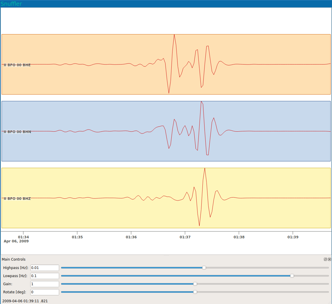
Example: Modelling Dynamic Waveforms

Example: Modelling Static Displacements

import os
import matplotlib.pyplot as plt
import numpy as np
from pyrocko import gf

KM2M = 1.0e3

# Download the GF store if it's not been done yet.
store_id = 'ak135_static_dgg'
if not os.path.exists(store_id):
    gf.ws.download_gf_store(
        site='kinherd', store_id=store_id)

# Finite source (rectangular fault)
rect_source = gf.RectangularSource(
    lat=31.0, lon=44.0, depth=5*KM2M,
    strike=104.0, dip=90.0, rake=5.0,
    length=8*KM2M, width=3*KM2M, slip=1.3)

# GNSS target (GPS stations)
norths = np.linspace(-20*KM2M, 20*KM2M, 100)
easts = np.linspace(-20*KM2M, 20*KM2M, 100)
north_shifts, east_shifts = np.meshgrid(norths, easts)

n_grids = 100 * 100
lats = np.ones(n_grids) * rect_source.lat
lons = np.ones(n_grids) * rect_source.lon

gnss_target = gf.GNSSCampaignTarget(
    lats=lats, lons=lons, north_shifts=north_shifts,
    east_shifts=east_shifts, quantity='displacement',
    store_id=store_id)

# Synthetic displcement calculation
engine = gf.LocalEngine(store_superdirs=['.'])
response = engine.process(rect_source, [gnss_target])
results = response.static_results()[0].result
                        

Example: Modelling Static Displacements

def plot_static_results(results, target):
    """Helper function for plotting displcements"""

    northings = target.coords5[:, 2]
    eastings = target.coords5[:, 3]

    fig, axes = plt.subplots(
        nrows=1, ncols=3, sharey=True, figsize=(13, 3))

    components = sorted(results.keys())
    for comp, ax in zip(components, axes):
        cmap = ax.scatter(
            eastings, northings, c=results[comp], s=15)
        ax.set(
            title=comp, xlabel='Easting [m]',
            ylabel='Northing [m]', aspect='equal')
        ax.ticklabel_format(
            axis='both', style='sci', scilimits=(0, 0))
        fig.colorbar(cmap, ax=ax)

    return fig
                        

Example: Modelling Static Displacements

                        # Plot synthetic displcements
                        fig = plot_static_results(results, gnss_target)
                        fig.savefig('syn_surfdisps.png')
                    

Grond

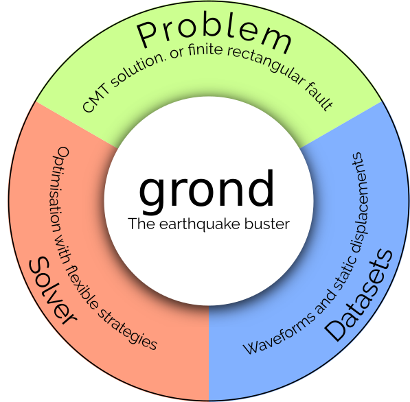
A probabilistic earthquake source joint inversion framework.

Invert your data with a few simple steps

                            # Create the example project with:
                            grond init example_regional_cmt grond-playground-regional/
                            cd grond-playground-regional/

                            # Download seismic waveform data:
                            bin/grondown_regional.sh gfz2018pmjk
                            # Download Green's function database:
                            bin/download_gf_stores.sh

                            # optional check the configuration and data:
                            grond check config/regional_cmt.gronf

                            # Run the optimization:
                            grond go config/regional_cmt.gronf

                            # Visualization of results report in browser:
                            grond report -so runs/cmt_gfz2018pmjk.grun
                        

Grond is configured in .gronf YAML files

													config/regional_cmt.gronf
												

													dataset_config: !grond.DatasetConfig
													  stations_stationxml_paths:
													  - 'data/events/${event_name}/waveforms/stations.geofon.xml'

													  events_path: 'data/events/${event_name}/event.txt'

													  waveform_paths: ['data/events/${event_name}/waveforms/raw']

													  blacklist: ['GE.UGM', 'GE.PLAI']
												

													problem_config: !grond.CMTProblemConfig
													    # Time relative to hypocenter origin time [s]
													    time: '-10 .. 10 | add'

													    # Centroid location with respect to hypocenter origin [m]
													    north_shift: '-15e3 .. 15e3'
													    east_shift: '-15e3 .. 15e3'
													    depth: '5e3 .. 30e3'

													    # Range of magnitudes to allow
													    magnitude: '5.7 .. 6.2'
												

                        optimiser_config: !grond.HighScoreOptimiserConfig
                        nbootstrap: 100

                        sampler_phases:

                        - !grond.UniformSamplerPhase
                            # Number of iterations
                            niterations: 1000

                        - !grond.DirectedSamplerPhase
                            # Number of iterations
                            niterations: 20000
                    

Single chain

Model uncertainties from Bayesian Bootstrapping

More example projects

Why Kite?

Bridging powerful InSAR processors with geophysical modelling frameworks

Quadtree Creation

Down-sampling of high-resolution InSAR scenes (Lossy Data Compression)

APS Correction

Removing atmospheric phase screen (APS) from displacement.
Empirically and from GACOS models.

Covariance Calculation

Data noise is mostly influenced by the ionosphere, atmosphere and decorrelation.

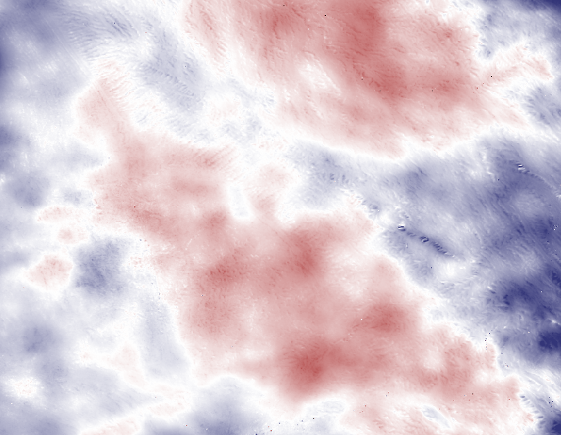
Noise is quantified by distance-dependent covariance and intrinsic variance at (d=0)

APS Correction

1. from regional atmospheric models (GACOS¹)
2. from topographic correlation (data-driven)

¹Yu C. et al., 2018

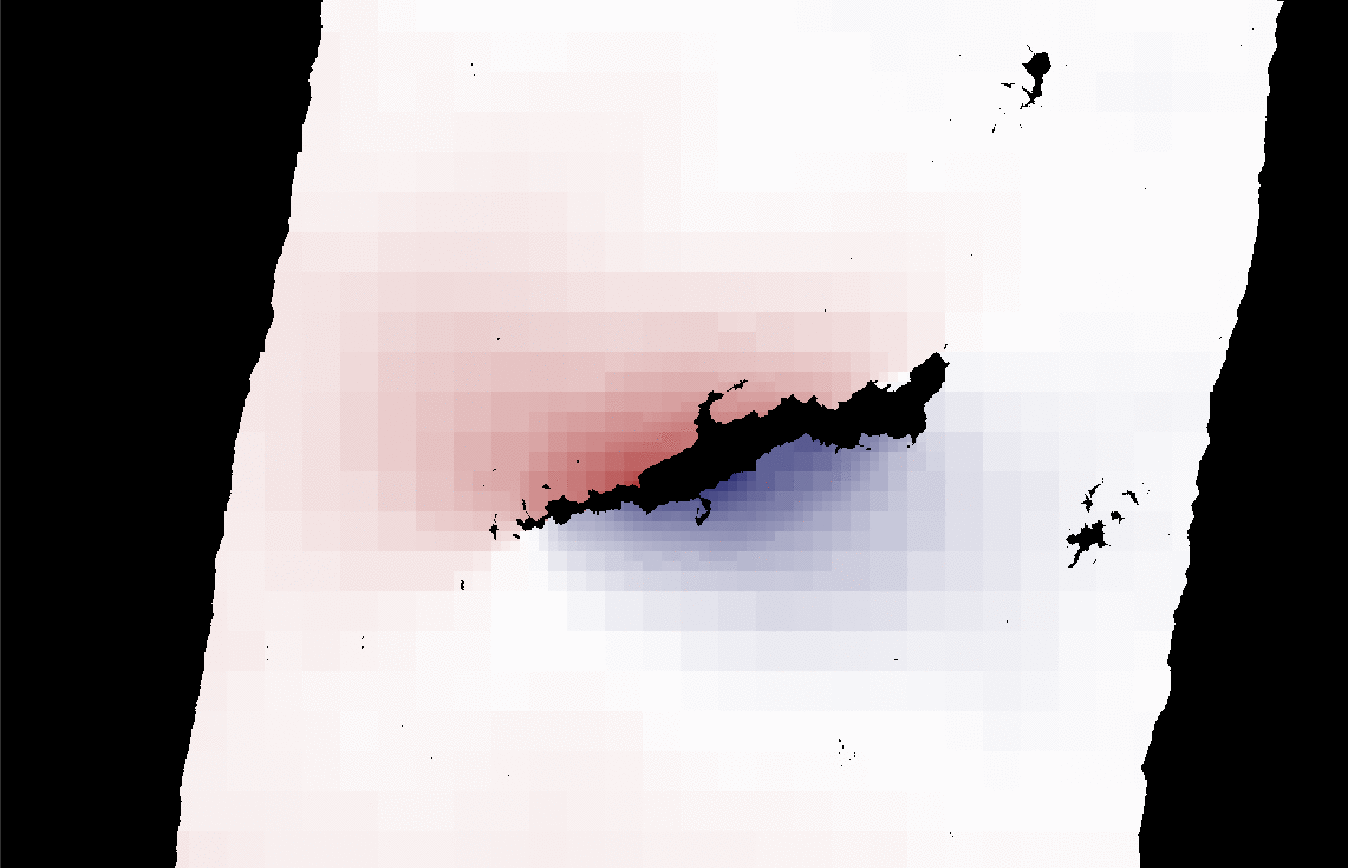
Modelling a salt cavern in Kiel, SH

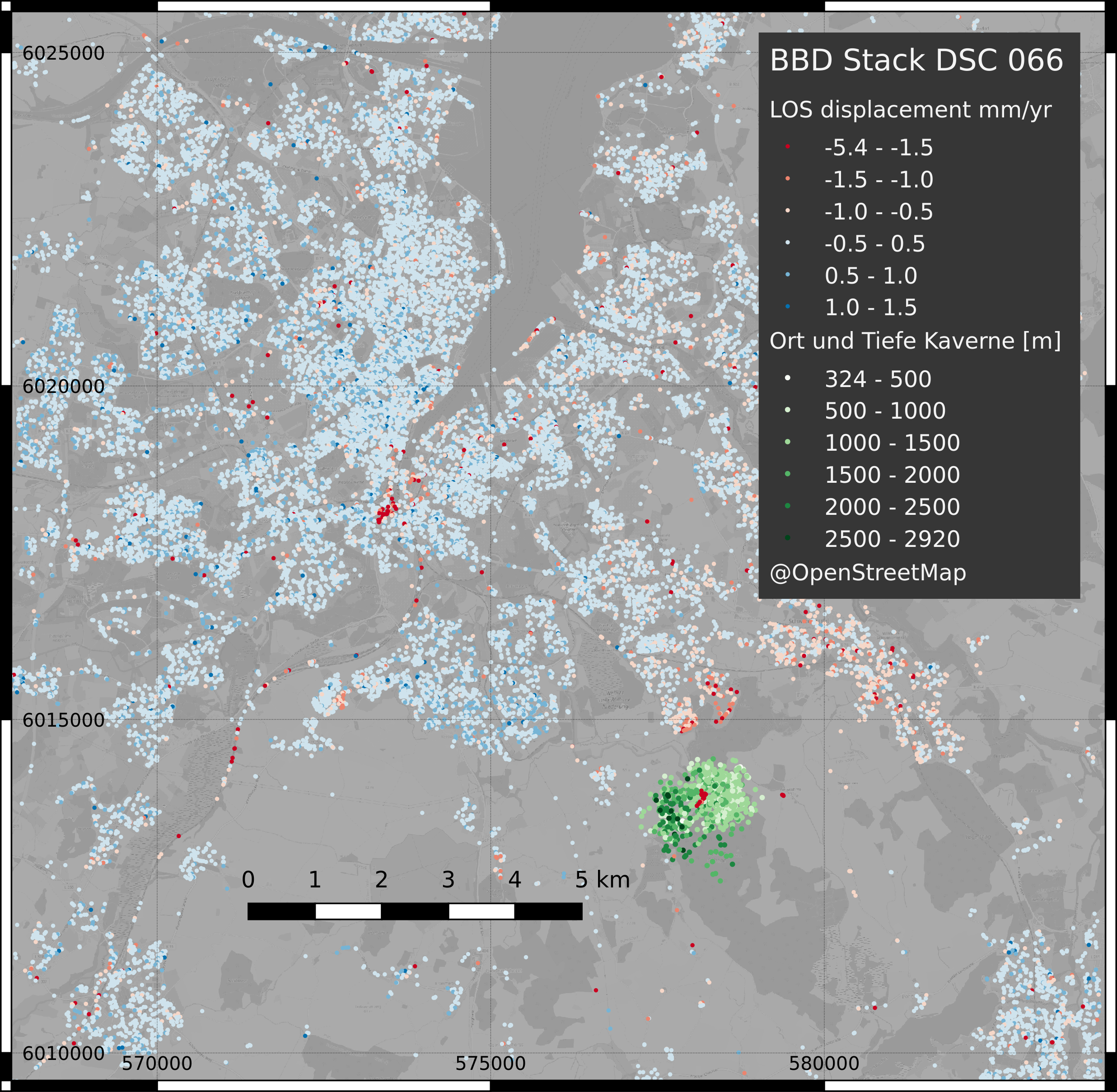
Modelling a salt cavern in Kiel, SH

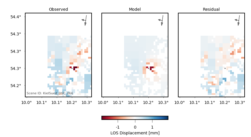
Key points

Pyrocko Sparrow

A bird's-eye view.

What is it?

• A simple geo-viewer.
• Desktop app.
• Interactive and snappy.
• For seismologists (mostly).
• Not complete and not released yet!

Objectives

• Earthquake locations

Objectives

• Earthquake locations
• Many Earthquake locations

Objectives

• Earthquake locations
• Many Earthquake locations
• MANY Earthquake locations

• Finite fault models I

• Finite fault models I
• Finite fault models II, kinematic rupture for 2009 L'Aquila from BEAT

• GEM active faults database

• Focal mechanism symbols (beachballs)

• Multi-resolution topography ETOPO + SRTM
• Offline

The Sparrow is user friendly!

Pyrocko Squirrel

Prompt seismological data access with a fluffy tail.

Wouldn't it be nice if...

Snuffler could handle 1M files?

• and could still instantly start up?
• respond as snappy as always?

Pyrocko's Pile could handle meta-data?

• providing instrument corrected seismograms?
• and rotated data?
• station epoch aware?

You wouldn't need any download scripts?

• Because your app can query online?
• Just when it needs the data?
• Be aware of what's available?
• It could incrementally fill up gaps?

Your event catalog would automatically sync with upstream?

Squirrel Example

from pyrocko import util
from pyrocko.squirrel import Squirrel

days = 60.*60.*24
tmin = util.stt('2009-04-06 00:00:00')
tmax = util.stt('2009-04-07 00:00:00')

sq = Squirrel()
sq.add('local/data')
sq.add_catalog('geofon', expires=30*days)
sq.add_fdsn('ingv', query_args=dict(network='IV', channel='HH?'))

sq.update(tmin=tmin, tmax=tmax)
sq.update_waveform_promises(tmin=tmin, tmax=tmax)

events = sq.get_events(magnitude_min=6.0)
stations = sq.get_stations()
channels = sq.get_channels()
responses = sq.get_responses()
traces = sq.get_waveforms(
    quantity='velocity', fmin=0.01, fmax=10.0,
    tmin=tmin, tmax=tmax)

sq.snuffle()
                        

Coming soon!

Pyrocko Squirrel will offer:

• Prompt,
• lazy,
• indexing,
• caching,
• dynamic

seismological dataset access.

Here's how it works...

    from pyrocko import squirrel
    sq = squirrel.Squirrel()
                        

    from pyrocko import squirrel
    sq = squirrel.Squirrel()
                        

    sq.add(['data.mseed', 'stations.xml'])  # content indexed
    sq.add('events.txt')
                        

    sq.add(['data.mseed', 'stations.xml'])
    sq.add('events.txt')
                        

    sq.get_stations()  # -> list of all station objects
    sq.get_station(codes='*.STA23.*.*')  # -> matching station
                        

    sq.get_stations()  # -> list of all station objects
    sq.get_station(codes='*.STA23.*.*')  # -> matching station
                        

    sq.remove('stations.xml')  # only from live selection
    sys.exit()
                        

    sq.remove('stations.xml')  # only from live selection
    sys.exit()  # app quits, database persists
                        

    sq = Squirrel()  # second start of app
    sq.add('data.mseed')
                        

    sq = Squirrel()
    sq.add('data.mseed')  # checks for modifications
                        

    sq = Squirrel()
    sq.add('data.mseed')  # updates index as needed
                        

    sq = Squirrel()
    sq.add('data.mseed', check=False)  # only index if unknown
                        

    sq = Squirrel()  # other app
    sq.add('stations.xml')  # selection is private by default
                        

    sq = Squirrel(persistent='S1')  # use selection named "S1"
    sq.add('data.mseed')
                        

    sq.add_fdsn_source('geofon', query_args={'network': 'GE'})
    sq.update(tmin=tmin, tmax=tmax)
                        

    sq.add_fdsn_source('geofon', query_args={'network': 'GE'})
    sq.update(tmin=tmin, tmax=tmax)  # update for time range
                        

    sq.add_fdsn_source('geofon', query_args={'network': 'GE'},
                       expires=3600.)  # expires in 1h
                        

    sq.update_waveform_promises(tmin=tmin, tmax=tmax)
    traces = sq.get_waveforms(tmin=tmin, tmax=tmax)
                        

    sq.update_waveform_promises(tmin=tmin, tmax=tmax)
    trs = sq.get_waveforms(tmin=tmin, tmax=tmax, codes='STA1')
                        

    sq.update_waveform_promises(tmin=tmin, tmax=tmax)
    trs = sq.get_waveforms(tmin=tmin, tmax=tmax, codes='STA1')
                        

    sq.update_waveform_promises(tmin=tmin, tmax=tmax)
    trs = sq.get_waveforms(tmin=tmin, tmax=tmax, codes='STA1')
                        

Pyrocko Ecosystem

Outlook